Visualize SPEXone L2 aerosol product (RemoTAP)

Visualize SPEXone L2 aerosol product (RemoTAP)#

Authors: Meng Gao (NASA, SSAI), Sean Foley (NASA, MSU), Guangliang Fu (SRON)

An Earthdata Login account is required to access data from the NASA Earthdata system, including NASA ocean color data.

Summary#

This notebook explores the SPEXone Level 2 (L2) aerosol product derived from the joint aerosol and surface retrieval algorithm: RemoTAP (Remote Sensing of Trace Gases and Aerosol Products algorithm). For more detailed information about the algorithm, please refer to the relevant documentation.

Similar to the HARP2 notebook, we analyze a scene from the Los Angeles wildfire, which includes both smoke and dust events (as observed by OCI and HARP2). However, due to the narrow swath of SPEXone data, the dust event will be the main focus of this tutorial. We will evaluate aerosol optical depth, aerosol absorption, and particle size information.

Learning Objectives#

By the end of this notebook, you will understand:

How to acquire SPEXone L2 data
What aerosol products are available
How to visualize basic aerosol properties
How to evaluate data quality

Contents#

Setup
Get Level-2 Data
Understanding SPEXone L2 product structure
Visulize SPEXone L2 aerosol properties
Improve data quality: filter low AOD pixels
Advanced quality assessment
Optional: Multi-angle data mask for cloud and data screening
Optional: pixel level uncertainty estimation
Reference

1. Setup#

Begin by importing all of the packages used in this notebook. If your kernel uses an environment defined following the guidance on the tutorials page, then the imports will be successful.

import cartopy.crs as ccrs
import earthaccess
import matplotlib.pyplot as plt
import numpy as np
import xarray as xr

auth = earthaccess.login(persist=True)

back to top

2. Get Level-2 Data#

SPEXone L2 data is available on both OB.DAAC and earth data cloud. Please refer L1C notebook on the access of cloud. The following block retrieves a single SPEXOne granule.

results = earthaccess.search_data(
    short_name="PACE_SPEXONE_L2_AER_RTAPOCEAN",
    temporal=("2025-01-09T20:00:20", "2025-01-09T20:00:21"),
    count=1,
)
paths = earthaccess.open(results)

PACE polarimeter L2 products for both HARP2 and SPEXone include four data groups

geolocation_data
geophysical_data
diagnostic_data
sensor_band_parameters

Here we merge all the data group together for convenience in data manipulations.

back to top

4. Visulize SPEXone L2 aerosol properties#

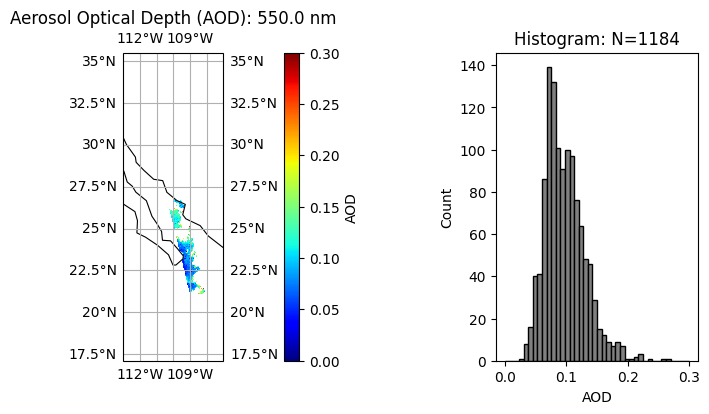
In this example, we visualize the aerosol properties for a scene during LA wild fire with both smoke and dust events. We read the total aerosol optical depth, single scattering albedo, and fine mode volume fraction as below:

aot = dataset["aot"].values
ssa = dataset["ssa"].values
fvf = dataset["fvf"].values
aot.shape, ssa.shape, fvf.shape

((395, 29, 18), (395, 29, 18), (395, 29))

We also need the spatial and angle dimensions as below:

lat = dataset["latitude"].values
lon = dataset["longitude"].values
plot_range = [lon.min(), lon.max(), lat.min(), lat.max()]
wavelength = dataset["wavelength3d"].values
print(wavelength)

[ 340.  355.  380.  440.  490.  500.  532.  550.  565.  670.  675.  765.
  865.  870. 1020. 1064. 1600. 2000.]

For future L2 product, the wavelength variable will be called simple wavelength, rather than wavelength_3d or wavelength3d

def plot_l2_product(
    data, plot_range, label, title, vmin, vmax, figsize=(12, 4), cmap="viridis"
):
    """Make map and histogram (default)"""

    # Create a figure with two subplots: 1 for map, 1 for histogram
    fig = plt.figure(figsize=figsize)
    gs = fig.add_gridspec(1, 2, width_ratios=[3, 1], wspace=0.3)

    # Map subplot
    ax_map = fig.add_subplot(gs[0], projection=ccrs.PlateCarree())
    ax_map.set_extent(plot_range, crs=ccrs.PlateCarree())
    ax_map.coastlines(resolution="110m", color="black", linewidth=0.8)
    ax_map.gridlines(draw_labels=True)

    # Assume lon and lat are defined globally or passed in
    pm = ax_map.pcolormesh(
        lon, lat, data, vmin=vmin, vmax=vmax, transform=ccrs.PlateCarree(), cmap=cmap
    )
    plt.colorbar(pm, ax=ax_map, orientation="vertical", pad=0.1, label=label)
    ax_map.set_title(title, fontsize=12)

    # Histogram subplot
    ax_hist = fig.add_subplot(gs[1])
    flattened_data = data[~np.isnan(data)]  # Remove NaNs for histogram
    valid_count = np.sum(~np.isnan(flattened_data))
    ax_hist.hist(
        flattened_data, bins=40, color="gray", range=[vmin, vmax], edgecolor="black"
    )
    ax_hist.set_xlabel(label)
    ax_hist.set_ylabel("Count")
    ax_hist.set_title("Histogram: N=" + str(valid_count))

    # plt.tight_layout()
    plt.show()

wavelength_index = 7
title = "Aerosol Optical Depth (AOD): " + str(wavelength[wavelength_index]) + " nm"
label = "AOD"
data = aot[:, :, wavelength_index]
plot_l2_product(
    data, plot_range=plot_range, label=label, title=title, vmin=0, vmax=0.3, cmap="jet"
)

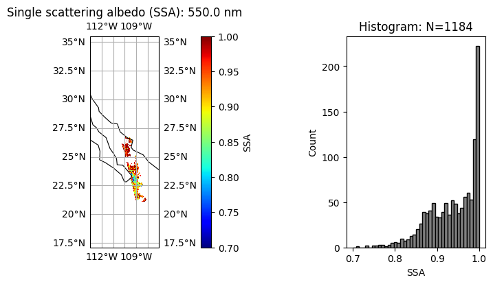
../../_images/3237f4ea112c853f9428c3a161292f96fd766c4ab7479efdf35558d03e27d3fe.png

wavelength_index = 7
title = "Single scattering albedo (SSA): " + str(wavelength[wavelength_index]) + " nm"
label = "SSA"
data = filtered_ssa = np.where(
    aot[:, :, wavelength_index] > 0.1, ssa[:, :, wavelength_index], np.nan
)
data = ssa[:, :, wavelength_index]
plot_l2_product(
    data, plot_range=plot_range, label=label, title=title, vmin=0.7, vmax=1, cmap="jet"
)

../../_images/05de12dffd9e6ddbcdc7f8a8dc66528c31345a4014b1718ac8d8beeec000f0e3.png

wavelength_index = 7
title = "Fine mode fraction"
label = "FVF"
data = fvf
plot_l2_product(
    data, plot_range=plot_range, label=label, title=title, vmin=0, vmax=1, cmap="jet"
)

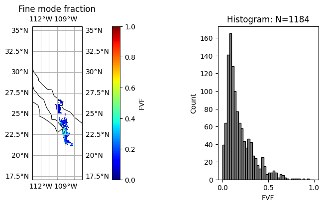
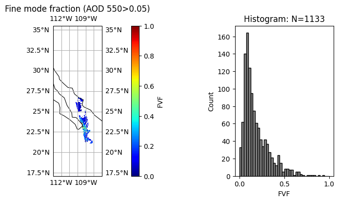
../../_images/0cd0d48e2a149bb9fb67b1dc297c2add7636c29c839acb105cb049853a5da176.png

We can clearly see the aerosol event with less absorption (high SSA) and large size (low FVF), probably dust.

back to top

5. Improve data quality: filter low AOD pixels#

Aerosol absorption and microphysics have larger uncertainties when aerosol loading is low. User can further remove low AOD cases when necessary.

wavelength_index = 7
aot_min = 0.05
title = (
    "Filtered single scattering albedo (SSA): "
    + str(wavelength[wavelength_index])
    + " nm (AOD 550>"
    + str(aot_min)
    + ")"
)
label = "SSA"
data = filtered_ssa = np.where(
    aot[:, :, wavelength_index] >= aot_min, ssa[:, :, wavelength_index], np.nan
)
plot_l2_product(
    data, plot_range=plot_range, label=label, title=title, vmin=0.7, vmax=1, cmap="jet"
)

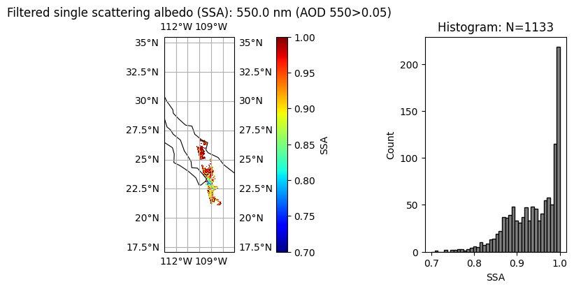
../../_images/a998284608dcb481f72cba67dfeb6be8a5b39a9d9d274ad9ed6fe57c2a3d464a.png

The difference in appearance (after matplotlib automatically normalizes the data) is negligible, but the difference in the physical meaning of the array values is quite important.

wavelength_index = 7
aot_min = 0.05
title = "Fine mode fraction (AOD 550>" + str(aot_min) + ")"
label = "FVF"
data = filtered_ssa = np.where(aot[:, :, wavelength_index] >= aot_min, fvf, np.nan)
plot_l2_product(
    data, plot_range=plot_range, label=label, title=title, vmin=0, vmax=1, cmap="jet"
)

../../_images/4363e2624aa5f858c1cc381cc9e6c505f6b1cbfc3c54e8907d8917f0ed8519b1.png

back to top

6. Advanced quality assessment#

Since the retrieval algorithm is based on optimal estimation by minimizing a \(\chi^2\) cost function defined as the difference between measurement (m) and forward model fitting (f), normalized by total uncertainties (\(\sigma\)).

\(\chi^2 = \frac{1}{N} \sum (f - m)^2/\sigma^2\)

Here N is the total number of measureents used in retreival. The \(\chi^2\) and \(N\) can be used to evaluate retrieval performance, the pixels with small \(\chi^2\) (good fitting) and large \(N\) (more pixels can be fitted) will better quality. A more quantitatively approach based on error propogation are used to compute retrieval uncertainty, which are also included for many of the data product. Note that RemoTAP algorithm do not adaptively remove measurements during retrieval, but instead all the measureemts as defined in the input file are used.

To support L3 data processing, a quality flag is also defined, which is usually based on \(\chi^2\) for SPEXone data. Other flags based on land-water adjacent, cloud ajacent are also included.

flag_0 : good.
flag_1 : large chi2.
flag_2 : land-water adjacent.
flag_3 : cloud adjacent.
flag_12 : large chi2, land-water adjacent.
flag_13 : large chi2, cloud adjacent.
flag_23 : land-water adjacent, cloud adjacent.
flag_123 : large chi2, land-water adjacent, cloud adjacent

Specifically for quality flag 0 and 1:

quality_flag = 0: when \(\chi^2<5\) over land and \(\chi^2<10\) over ocean, not land-water-adjacent, not cloud-adjacent
quality_flag = 1: when \(\chi^2 \ge 5\) over land and \(\chi^2 \ge 10\) over ocean

chi2 = dataset["chi2"].values
quality_flag = dataset["quality_flag"].values

title = r"Retrieval cost function: $\chi^2$"
label = r"$\chi^2$"
data = chi2
plot_l2_product(
    data, plot_range=plot_range, label=label, title=title, vmin=0, vmax=3, cmap="jet"
)

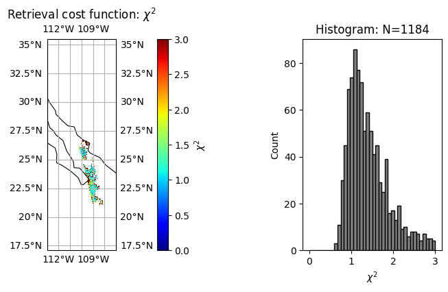
../../_images/e67f2dbceabc4276506acf1a7792796955137d724af56bfc9c08ad58711f4bd2.png

np.nanmean(chi2)

np.float32(3.0640965)

Note that \(\chi^2\) converges reasonably well with peak at 1. There are also pixels which do not converge well with relatively high cost function. These pixels need to be removed for more detailed analysis.

title = "Retrieval quality flag"
label = "quality_flag"
data = quality_flag
plot_l2_product(
    data, plot_range=plot_range, label=label, title=title, vmin=0, vmax=3, cmap="cool"
)

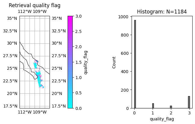
../../_images/a000720f8a9ed6940cdcd9ec713e35698ca699a01f48b74e7ebbce4077a26303.png

We can evaluate quality flag based on the \(\chi^2\) and \(N\), and most pixels have reach to the best quality with quality_flag=0.

back to top

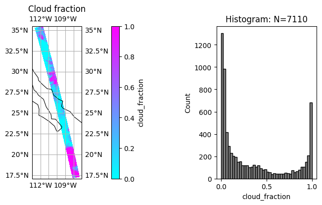
7 [Optional] Cloud fraction#

RemoTAP conducted cloud masking based on an internal neural network model. The cloud fraction (CF) can be evaluated as follows: CF<0.05 is considered as clear sky, the others are as cloudy.

cloud_fraction = dataset["cloud_fraction"].values
cloud_fraction.shape

(395, 29)

title = "Cloud fraction"
label = "cloud_fraction"
data = cloud_fraction
plot_l2_product(
    data, plot_range=plot_range, label=label, title=title, vmin=0, vmax=1, cmap="cool"
)

../../_images/27d0c5d98af52b7187dccd4c604a9a6dc6c444e7c2efe7aa170fe7c70e580458.png

back to top

8. Optional: pixel level uncertainty estimation#

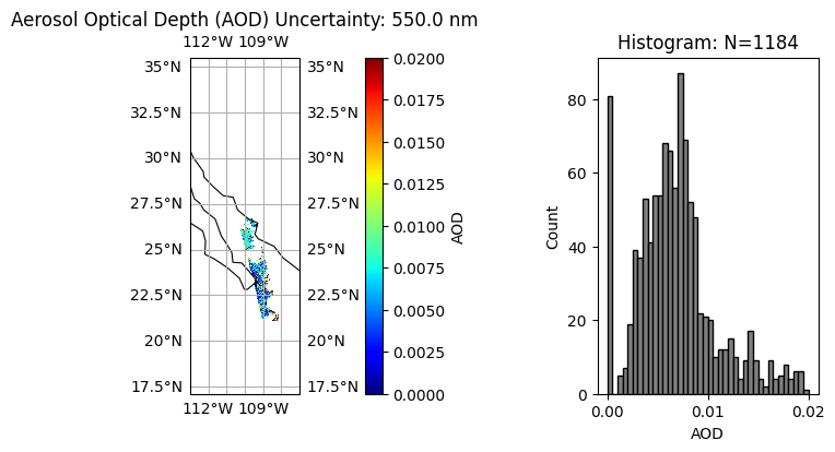
As mentioned previously, pixel level uncertainty can be evalated through error propagation, which propgation measurement uncertainty through Jacobian of the forward model. The estimated uncertainties are availalbe in the SPEXone RemmoTAP product. Here we look at the uncertainties of AOD.

aot_unc = dataset["aot_uncertainty"].values
aot_unc.shape

(395, 29, 18)

wavelength_index = 7
title = (
    "Aerosol Optical Depth (AOD) Uncertainty: "
    + str(wavelength[wavelength_index])
    + " nm"
)
label = "AOD"
data = aot_unc[:, :, wavelength_index]
plot_l2_product(
    data, plot_range=plot_range, label=label, title=title, vmin=0, vmax=0.02, cmap="jet"
)

../../_images/f81f4f33aabd19ec73647278bd26ea6dd6375a5dea5e992e9f2c599e0387c30e.png

plt.figure(figsize=(8, 4))
plt.plot(aot[:, :, wavelength_index], aot_unc[:, :, wavelength_index], "b.", alpha=0.3)
plt.ylim(0, 0.02)
plt.xlim(0, 0.3)
plt.xlabel("AOD")
plt.ylabel("AOD Uncertainty")

Text(0, 0.5, 'AOD Uncertainty')

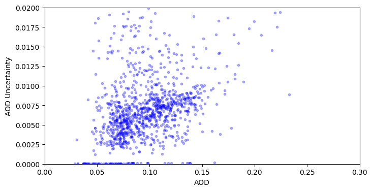
../../_images/26cdf54c2df117d33dafa80fffd4b601f8a589c4edd537e09abbfc9a9955df4e.png

As shown above, the AOD uncertainties increase with the AOD value. You can play with other retrieval uncertainties and evaluate how they vary with AOD.

back to top

9. Reference#

Guangliang Fu, Jeroen Rietjens, Raul Laasner, Laura van der Schaaf, Richard van Hees, Zihao Yuan, Bastiaan van Diedenhoven, Neranga Hannadige, Jochen Landgraf, Martijn Smit, Kirk Knobelspiesse, Brian Cairns, Meng Gao, Bryan Franz, Jeremy Werdell, Otto Hasekamp (2025). Aerosol retrievals from SPEXone on the NASA PACE mission: First results and validation. Geophysical Research Letters, 52, e2024GL113525. https://doi.org/10.1029/2024GL113525

back to top

Visualize SPEXone L2 aerosol product (RemoTAP)

Contents

Visualize SPEXone L2 aerosol product (RemoTAP)#

Summary#

Learning Objectives#

Contents#

1. Setup#

2. Get Level-2 Data#

3. Understanding SPEXone L2 product structure#

4. Visulize SPEXone L2 aerosol properties#

5. Improve data quality: filter low AOD pixels#

6. Advanced quality assessment#

7 [Optional] Cloud fraction#

8. Optional: pixel level uncertainty estimation#

9. Reference#