
Orientation to PACE/OCI Terrestrial Products#
Tutorial Lead: Skye Caplan (NASA, SSAI)
An Earthdata Login account is required to access data from the NASA Earthdata system, including NASA ocean color data.
Summary#
This notebook introduces the Level-2 files containing the surface reflectance product from the Ocean Color Instrument (OCI) on board the PACE satellite. The visualizations rely on flags accompanying the data variables that enable masking for features more relevant to terrestrial data products. The notebook highlights the hyperspectral-enabled vegetation indices (VIs) made possible by the high spectral resolution of OCI.
Learning objectives#
By the end of this tutorial you will be able to:
Open OCI surface reflectance products
Mask features you can ignore using built-in flags
Compare VIs developed using different spectral features
Contents#
1. Setup#
We begin by importing the packages used in this notebook. At first glance, the cf_xarray package appears unused and should therefore not be imported. Since it actually provides the cf attribute used below on certain xarray data structures, we indicate that the import is necessary by the inline comment # noqa: F401 referencing rule F401. Likewise for hvplot.xarray and the hvplot attribute.
import cartopy
import cf_xarray  # noqa: F401
import earthaccess
import hvplot.xarray  # noqa: F401
import matplotlib.pyplot as plt
import xarray as xr

crs = cartopy.crs.PlateCarree()
2. Search and Open Surface Reflectance Data#
Set and persist your Earthdata login credentials.
auth = earthaccess.login(persist=True)
We will use earthaccess to open a Level-2 surface reflectance granule that covers part of the Great Lakes region of North America. When fetching one specific granule, use the concept_id argument to provide a unique identifier looked up elsewhere.
results = earthaccess.search_data(
    short_name="PACE_OCI_L2_SFREFL",
    granule_name="*.20240701T175112.*",
)
for item in results:
    display(item)

paths = earthaccess.open(results)
We use xr.open_datatree() to access all “groups” of variables (a.k.a. “datasets”) within a NetCDF file. It will be easier to work with a single dataset, which we create by merging the data and coordinate variables we need from different groups. Longitude and latitude appear as data variables, however, so they must be explicitly set as coordinates.
datatree = xr.open_datatree(paths[0])
dataset = xr.merge(
    (
        datatree.ds,
        datatree["geophysical_data"].ds[["rhos", "l2_flags"]],
        datatree["sensor_band_parameters"].coords,
        datatree["navigation_data"].ds.set_coords(("longitude", "latitude")).coords,
    )
)
dataset
<xarray.Dataset> Size: 1GB
Dimensions:        (number_of_lines: 1710, pixels_per_line: 1272,
                    wavelength_3d: 122)
Coordinates:
  * wavelength_3d  (wavelength_3d) float64 976B 346.0 351.0 ... 2.258e+03
    longitude      (number_of_lines, pixels_per_line) float32 9MB ...
    latitude       (number_of_lines, pixels_per_line) float32 9MB ...
Dimensions without coordinates: number_of_lines, pixels_per_line
Data variables:
    rhos           (number_of_lines, pixels_per_line, wavelength_3d) float32 1GB ...
    l2_flags       (number_of_lines, pixels_per_line) int32 9MB ...
Attributes: (12/45)
    title:                             OCI Level-2 Data SFREFL
    product_name:                      PACE_OCI.20240701T175112.L2.SFREFL.V3_...
    processing_version:                3.0
    history:                           l2gen par=/data6/sdpsoper/vdc/vpu25/wo...
    instrument:                        OCI
    platform:                          PACE
    ...                                ...
    geospatial_lon_max:                -63.882717
    geospatial_lon_min:                -99.1249
    startDirection:                    Ascending
    endDirection:                      Ascending
    day_night_flag:                    Day
earth_sun_distance_correction: 0.9674437642097473In the above display of our Level-2 file, we have the data variables rhos and l2_flags. The rhos variable are surface reflectances, and the l2_flags are quality flags as defined by the Ocean Biology Processing Group (OBPG).
We can also see which wavelengths we have surface reflectance measurements at by accessing the wavelength_3d coordinate:
dataset["wavelength_3d"]
<xarray.DataArray 'wavelength_3d' (wavelength_3d: 122)> Size: 976B
array([ 346.,  351.,  356.,  361.,  366.,  371.,  375.,  380.,  385.,  390.,
        395.,  400.,  405.,  410.,  415.,  420.,  425.,  430.,  435.,  440.,
        445.,  450.,  455.,  460.,  465.,  470.,  475.,  480.,  485.,  490.,
        495.,  500.,  505.,  510.,  515.,  520.,  525.,  530.,  535.,  540.,
        545.,  550.,  555.,  560.,  565.,  570.,  575.,  580.,  586.,  615.,
        620.,  625.,  630.,  635.,  640.,  642.,  645.,  647.,  650.,  652.,
        655.,  657.,  660.,  662.,  665.,  667.,  670.,  672.,  675.,  677.,
        679.,  682.,  697.,  699.,  702.,  704.,  707.,  709.,  712.,  714.,
        719.,  724.,  729.,  734.,  739.,  742.,  744.,  747.,  749.,  752.,
        754.,  772.,  774.,  779.,  784.,  789.,  794.,  799.,  804.,  809.,
        814.,  819.,  824.,  829.,  835.,  840.,  845.,  850.,  855.,  860.,
        865.,  870.,  875.,  880.,  885.,  890.,  895., 1038., 1249., 1618.,
       2131., 2258.])
Coordinates:
* wavelength_3d (wavelength_3d) float64 976B 346.0 351.0 ... 2.258e+03
Attributes:
long_name: wavelengths
units: nm
valid_min: 0
valid_max: 20000Note that “wavelength_3d” is an indexed coordinate, which allows us to subset the dataset by slicing or choosing individual wavelengths. The method="nearest" argument lets us select one wavelength without knowning its exact value.
rhos_860 = dataset["rhos"].sel({"wavelength_3d": 860}, method="nearest")
Now we can plot surface reflectance at this one wavelength in the near-infrared (NIR), where land is bright and we can differentiate land, water, and clouds.
fig, ax = plt.subplots(figsize=(9, 5), subplot_kw={"projection": crs})
ax.gridlines(draw_labels={"left": "y", "bottom": "x"}, linewidth=0.25)
ax.coastlines(linewidth=0.5)
ax.add_feature(cartopy.feature.OCEAN, edgecolor="w", linewidth=0.01)
ax.add_feature(cartopy.feature.LAND, edgecolor="w", linewidth=0.01)
rhos_860.plot(x="longitude", y="latitude", cmap="Greys_r", vmin=0, vmax=1.0)
plt.show()
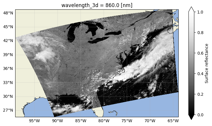
Great! We’ve plotted the surface reflectance at a single band for the whole scene. However, there are some features in this image that we want to exclude from our analysis.
3. Mask for Clouds and Water#
Level-2 files usually include information on the quality of each pixel in the scene, presented in the l2_flags variable. Let’s look at it a little more closely.
dataset["l2_flags"]
<xarray.DataArray 'l2_flags' (number_of_lines: 1710, pixels_per_line: 1272)> Size: 9MB
[2175120 values with dtype=int32]
Coordinates:
    longitude  (number_of_lines, pixels_per_line) float32 9MB ...
    latitude   (number_of_lines, pixels_per_line) float32 9MB ...
Dimensions without coordinates: number_of_lines, pixels_per_line
Attributes:
    long_name:      Level-2 Processing Flags
    valid_min:      -2147483648
    valid_max:      2147483647
    flag_masks:     [          1           2           4           8         ...
flag_meanings: ATMFAIL LAND PRODWARN HIGLINT HILT HISATZEN COASTZ SPARE ...At first glance, we can see that l2_flags is in the same shape as the surface reflectance we plotted above. The attributes look sort of meaningful, but also sort of like random numbers and abbreviations. If we were to plot l2_flags, the result wouldn’t look like anything useful at all. This is because the values in l2_flags include many quality flags compactly encoded in the binary representation of an integer. In order to use the flags applied to each pixel, we need a decoded representation. Since all OB.DAAC data follows the CF Metadata Conventions, we only need to import the cf_xarray package to access the decoded flags.
For example, say we want to mask any pixels flagged as clouds and/or water in our data. First, we have to make sure that the l2_flags variable is readable by cf_xarray so that we can eventually apply them to the data. We can check this using the built in is_flag_variable property.
dataset["l2_flags"].cf.is_flag_variable
True
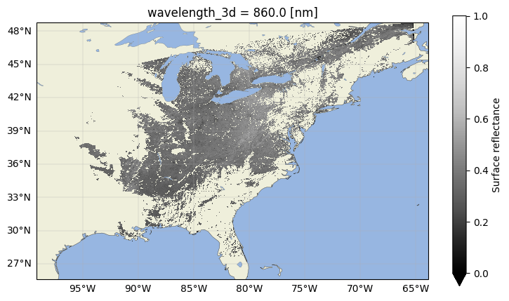
The statement returned True, which means l2_flags is recognized as a flag variable. By referencing the OBPG ocean color flags documentation, we find the names of the flags we want to mask out. In this case, “CLDICE” is the cloud flag, and while there is no specific water mask (this is an ocean mission, after all) there is a “LAND” flag we can invert to mask out water. The expressions in the cell below will retain any pixel identified as land which is also not a cloud (thanks to the ~).
cldwater_mask = (
    (dataset["l2_flags"].cf == "LAND")
    & ~(dataset["l2_flags"].cf == "CLDICE")
)
rhos = dataset["rhos"].where(cldwater_mask)
Note that we need to redefine the rhos_860 selection with the new masked dataset.
rhos_860 = rhos.sel({"wavelength_3d": 860}, method="nearest")
Then, we can see if the mask worked by plotting the data once again.
fig, ax = plt.subplots(figsize=(9, 5), subplot_kw={"projection": crs})
ax.coastlines(linewidth=0.25)
ax.gridlines(draw_labels={"left": "y", "bottom": "x"}, linewidth=0.25)
ax.add_feature(cartopy.feature.OCEAN, edgecolor="w", linewidth=0.01)
ax.add_feature(cartopy.feature.LAND, edgecolor="w", linewidth=0.01)
ax.add_feature(cartopy.feature.LAKES, edgecolor="k", linewidth=0.1)
rhos_860.plot(x="longitude", y="latitude", cmap="Greys_r", vmin=0, vmax=1.0)
plt.show()
4. Working with PACE Terrestrial Data#
Now that we have our surface reflectance data masked, we can start doing some analysis. A relatively simple but informative use of surface reflectance data is the calculation of vegetation indices (VIs). VIs use the well-known, idealized spectral shape of leaves and other materials to determine surface features contributing to a pixel. Vegetation health, relative water content, or even the presence of snow can be measured using VIs. These indices are particularly valuable when considering the limited number of bands in previous multispectral sensors, but they can of course be calculated with hyperspectral sensors like PACE.
Multispectral Vegetation Indices#
Let’s take NDVI for example. NDVI is a metric which quantifies plant “greenness”, which is related to the abundance and health of the vegetation in a pixel. It is a normalized ratio of the surface reflectance for red (\(\rho_{red}\)) and near-infrared (\(\rho_{NIR}\)) bands:
You’ll notice that the equation does not mention specific wavelengths, but rather just requires a “red” measurement and a “NIR” measurement. PACE provides many reflectance measurements throughout the red and NIR regions of the spectrum, as we can see in the plots below.
To visualize the spectra, we want to plot across the wavelength dimension of individual pixels, so we’ll take just a small sample from the dataset. We also like to separate the hyperspectral (ultraviolet to NIR wavelengths) and multispectral (NIR to SWIR wavelengths) regions when plotting spectra to better understand the spectral shapes.
sample_rhos = rhos.sel(
    {"number_of_lines": 900, "pixels_per_line": slice(None, None, 25)}
)
hyper_rhos = sample_rhos.sel({"wavelength_3d": slice(None, 895)})
multi_rhos = sample_rhos.sel({"wavelength_3d": slice(1038, None)})
fig, (a, b) = plt.subplots(1, 2, figsize=(10, 5), sharey=True)
hyper_rhos.plot.line("k", x="wavelength_3d", ax=a, alpha=0.3, add_legend=False)
multi_rhos.plot.line("k--o", x="wavelength_3d", ax=b, alpha=0.3, add_legend=False)
b.set_ylabel("")
plt.show()
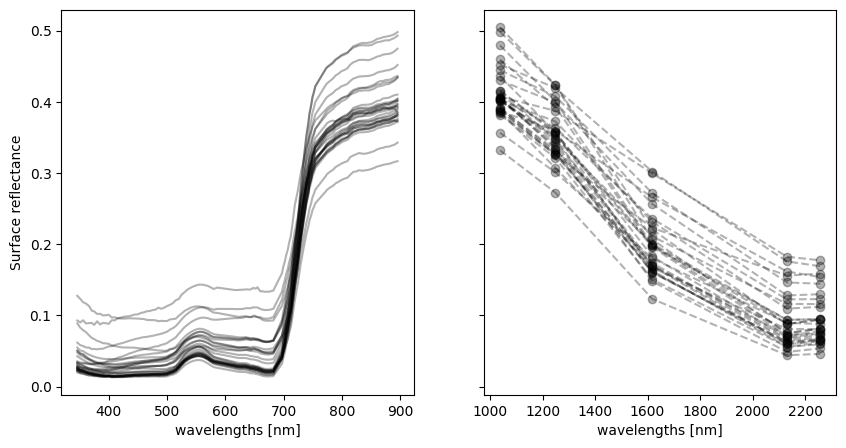
To calculate NDVI and other heritage multispectral indices with PACE, you could choose a single band from each region. However, doing so would mean capturing only the information from one of OCI’s narrow 5 nm bands. In other words, we would miss out on information from surrounding wavelengths that improve these calculations and would have otherwise been included from other sensors with broader bandwidths. To preserve continuity with those sensors and calculate a more comparable NDVI, we can take an average of several OCI bands to simulate a multispectral measurement, incorporating as much relevant information into the calculation as possible.
We’ll take MODIS’s red and NIR bandwidths and average the PACE measurements together.
rhos_red = rhos.sel({"wavelength_3d": slice(620, 670)}).mean("wavelength_3d")
rhos_nir = rhos.sel({"wavelength_3d": slice(840, 875)}).mean("wavelength_3d")
Now, we can use those averaged reflectances to calculate NDVI.
ndvi = (rhos_nir - rhos_red) / (rhos_nir + rhos_red)
ndvi.attrs["long_name"] = "Normalized Difference Vegetation Index (NDVI)"
fig, ax = plt.subplots(figsize=(9, 5), subplot_kw={"projection": crs})
ax.coastlines(linewidth=0.5)
ax.gridlines(draw_labels={"left": "y", "bottom": "x"}, linewidth=0.25)
ax.add_feature(cartopy.feature.OCEAN, edgecolor="w", linewidth=0.01)
ax.add_feature(cartopy.feature.LAND, edgecolor="w", linewidth=0.01)
ax.add_feature(cartopy.feature.LAKES, edgecolor="k", linewidth=0.1)
ndvi.plot(x="longitude", y="latitude", cmap="RdYlGn", vmin=-0.05, vmax=1.0)
ax.set_title("NDVI from PACE OCI")
plt.show()
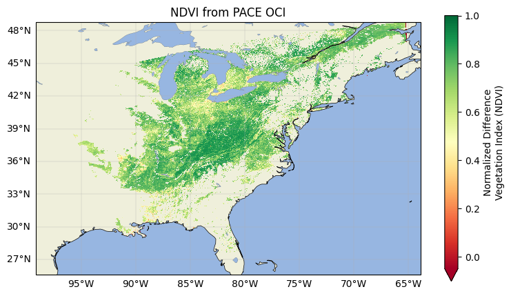
Making these heritage calculations are important for many reasons, not least of which is because the MODIS instruments are reaching the end of their lives and will soon be decommissioned. PACE can continue the time series of these VI datasets that would otherwise be lost. However, as a hyperspectral instrument, PACE/OCI is able to go beyond these legacy calculations and create new products, as well!
Hyperspectral-enabled Vegetation Indices#
Hyperspectral-enabled VIs are still band ratios, but rather than using wide bands to capture the general aspects of a spectrum, they target minute fluctuations in surface reflectances to describe detailed features of a pixel, such as relative pigment concentration in plants. This means that, unlike multispectral VIs, these indices require the narrow bandwidths inherent to OCI data. In other words, we don’t want to do any band averaging as we did above, because we’d likely dilute the very signal we want to pull out. The calculations for this type of VI are therefore even simpler.
We’ll take the Chlorophyll Index Red Edge (CIRE) as an example of a hyperspectral-enabled VI. CIRE uses bands from the red edge and the NIR to get at relative canopy chlorophyll content:
Because we’re not doing any averaging, all we have to do is grab the bands from our dataset and follow the equation. We’ll use the closest bands that the SFREFL suite has to 800 and 705 nm.
rhos_800 = rhos.sel({"wavelength_3d": 800}, method="nearest")
rhos_705 = rhos.sel({"wavelength_3d": 705}, method="nearest")

cire = (rhos_800 / rhos_705) - 1
cire.attrs["long_name"] = "Chlorophyll Index Red Edge (CIRE)"
We can compare these maps side by side to see similarities and differences in the patterns of each VI.
fig, (a, b) = plt.subplots(1, 2, figsize=(13, 4), subplot_kw={"projection": crs})
plot_args = {
    "x": "longitude",
    "y": "latitude",
    "cmap": "RdYlGn",
    "vmin": 0,
}
for ax in (a, b):
    ax.coastlines(linewidth=0.25)
    ax.gridlines(draw_labels={"left": "y", "bottom": "x"}, linewidth=0.25)
    ax.add_feature(cartopy.feature.OCEAN, edgecolor="w", linewidth=0.01)
    ax.add_feature(cartopy.feature.LAND, edgecolor="w", linewidth=0.01)
    ax.add_feature(cartopy.feature.LAKES, edgecolor="k", linewidth=0.1)
cire.plot(ax=a, **plot_args, vmax=6)
a.set_title("CIRE on July 1st, 2024")
ndvi.plot(ax=b, **plot_args, vmax=1)
b.set_title("NDVI on July 1st, 2024")
plt.subplots_adjust(wspace=0.1)
plt.show()
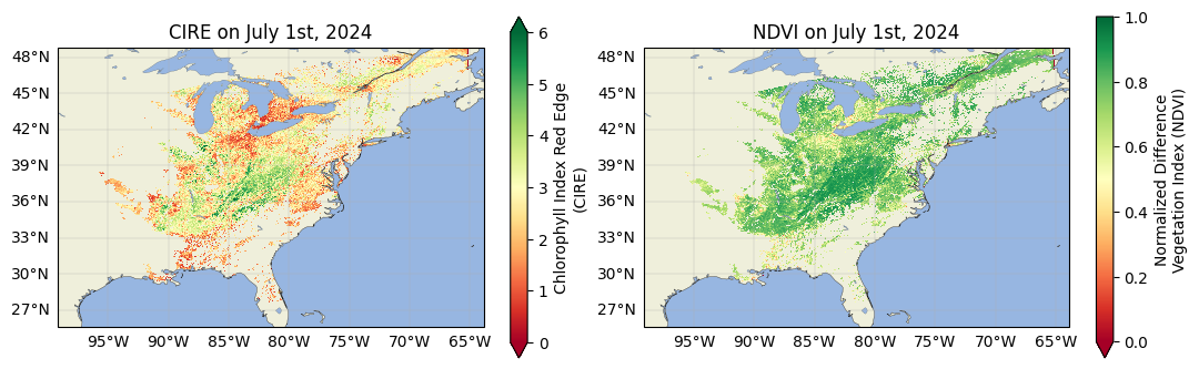
Comparing these two plots, we can see some similarities and differences. Generally, the patterns of high and low values fall in the same places - this is because NDVI is essentially measuring the amount of green vegetation, and CIRE is measuring the amount of green pigment in plants. However, CIRE also has a higher dynamic range than NDVI does. For one, NDVI saturates as vegetation density increases, so a wide range of ecosystems with varying amounts of green vegetation may have very similar NDVI values. On the other hand, CIRE is not as affected by the leaf area, and can instead hone in on the relative amount of chlorophyll pigment in a pixel rather than the amount of leaves. This is a major advantage of CIRE and other hyperspectral-enabled VIs like the Carotenoid Content Index (Car), enabling us to track specific biochemical shifts in plants that correspond to states of photosynthetic or photoprotective ability, and thus provide insight on plant physiological condition.
If calculating these indices manually felt a little tedious, not to worry! PACE/OCI provides 10 VIs in its LANDVI products available in Level-2 (short_name="PACE_OCI_L2_LANDVI") and Level-3 (short_name="PACE_OCI_L3M_LANDVI"). The suite includes 6 heritage indices and 4 narrowband pigment indices including CIRE. Read more about it in the LANDVI ATBD.
results = earthaccess.search_data(
    short_name="PACE_OCI_L3M_LANDVI",
    granule_name="*.20240701_20240731.*.0p1deg.*",
)
for item in results:
    display(item)
paths = earthaccess.open(results)
The Level-3 data products come binned and gridded on a global projection at multiple temporal and spatial resolutions. The granule shown here is a monthly, 0.1 degree aggregate. We’ll conclude by dropping in a nifty interactive visualization brought to you by the hvplot package.
dataset = xr.open_dataset(paths[0])
array = dataset.drop_vars("palette").to_array("Product")
array.attrs["long_name"] = "Vegetation Index"
array.hvplot(
    x="lon",
    y="lat",
    cmap="magma",
    aspect=2,
    title="July 2024 Monthly Average",
    rasterize=True,
    widget_location='top',
)
You have completed the notebook introducing terrestrial data products from OCI. We suggest looking at the notebook on “Satellite Data Visualization” for tips on making beautiful PACE/OCI images.