
Reprojecting and Formatting PACE OCI Data#
Authors: Skye Caplan (NASA, SSAI)
Last updated: July 28, 2025
An Earthdata Login account is required to access data from the NASA Earthdata system, including NASA PACE data.
Executing this notebook requires an instance with up to 8GB of memory.
Summary#
This notebook will use rioxarray to reproject PACE OCI data from the instrument swath into a projected coordinate system and save the file as a GeoTIFF (.tif), a common data format used in GIS applications.
Learning Objectives#
At the end of this notebook you will know how to:
Open PACE OCI surface reflectance and vegetation index products
Reproject those data into defined coordinate reference systems
Export those reprojected data as GeoTIFFs
Contents#
1. Setup#
Begin by importing all of the packages used in this notebook. Please ensure your environment has the most recent versions of rioxarray (>=0.19.0) and rasterio (>=1.4.3), as the functionality allowing us to correctly convert PACE Level-2 (L2) files to GeoTIFF is relatively new.
from pathlib import Path

import cartopy
import cartopy.crs as ccrs
import cf_xarray  # noqa: F401
import earthaccess
import matplotlib.pyplot as plt
import numpy as np
import rasterio
import rioxarray as rio
import xarray as xr
from rasterio.enums import Resampling
The goal of this tutorial is to reproject and convert Level-2 (L2) PACE OCI data between formats, but L2 PACE OCI data comes in many forms. We’ll cover two examples here - one with 3-dimensional surface reflectance (SFREFL) data, and one with 2-dimensional vegetation index (VI) data - to illustrate how these datasets need to be handled.
The following cells use earthaccess to set and persist your Earthdata login credentials, then search for and download the relevant datasets for a scene covering eastern North America.
auth = earthaccess.login(persist=True)

results = earthaccess.search_data(
    short_name=["PACE_OCI_L2_SFREFL", "PACE_OCI_L2_LANDVI"],
    granule_name="*20240701T175112*",
)
for item in results:
    display(item)


paths = earthaccess.download(results, local_path="data")
2. Reprojecting Level-2 PACE Data#
2.1. 2D Variables - Vegetation Indices#
All of PACE OCI’s L2 data are still in the instrument swath - in other words, they are not projected to any sort of regular grid, which makes comparing between satellites, or even between two PACE OCI granules in the same location, difficult. However, each pixel is geolocated (i.e., has an associated latitude and longitude), meaning we can reproject our data onto a grid to make working with it more intuitive.
As mentioned above, we’re working with two data products in this tutorial. We’ll open both as xarray datatrees and display their different dimensional architecture:
vi_path, sr_path = paths[0], paths[1]

sr_dt = xr.open_datatree(sr_path)
vi_dt = xr.open_datatree(vi_path)

print("Surface reflectance dimensions: ", sr_dt["geophysical_data"]["rhos"].dims)
print("Vegetation index dimensions: ", vi_dt["geophysical_data"]["cire"].dims)
Surface reflectance dimensions:  ('number_of_lines', 'pixels_per_line', 'wavelength_3d')
Vegetation index dimensions:  ('number_of_lines', 'pixels_per_line')
As we can see, the dimensions between the variables in both datasets differ. The surface reflectance contained in the rhos variable have 3 dimensions corresponding to (rows, columns, wavelength), while each VI variable (e.g., ndvi or cire) is a 2D variable with (row, column) dimensions.
If we plot one of these variables, we’ll see that they aren’t on any sort of regular spatial grid, and will instead be plotted by their row (number_of_lines) and column (pixels_per_line) indices as any non-geospatial array would be.
vi_dt["geophysical_data"]["cire"].plot(cmap="magma", vmin=0, vmax=5)
plt.show()
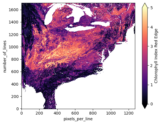
This is fine for a quick look into the data, but any analysis would be better served with a mapped dataset. Let’s start with VIs to illustrate the projection process. We’ll take the whole geophysical_data group as the source dataset for reprojection since each VI is contained in this group as a separate variable in the dataset.
The basic steps for reprojection are:
Mask for any quality issues or obscured pixels
Set the coordinates to the latitudes and longitudes from the
navigation_datagroupAssign the spatial dimensions as the columns (or the x coordinate,
pixels_per_line) and rows (or the y coordinate,number_of_lines)Assign the source Coordinate Reference System (CRS). Since we are working with unprojected PACE OCI lat/lons based on the WGS84 datum, we’ll use EPSG 4326 as our source CRS.
Use
rio.reprojectto project our source dataset
We can see in the plot above that the VI datasets come masked for water, but we should also mask out any cloudy pixels for a clean dataset as well. If we print out the geophysical_data group of either of our datasets, there will be a variable called l2_flags at the bottom of the list, in which the quality flag information is stored:
vi_src = vi_dt["geophysical_data"].to_dataset()
vi_src
<xarray.Dataset> Size: 96MB
Dimensions:   (number_of_lines: 1710, pixels_per_line: 1272)
Dimensions without coordinates: number_of_lines, pixels_per_line
Data variables:
    ndvi      (number_of_lines, pixels_per_line) float32 9MB ...
    evi       (number_of_lines, pixels_per_line) float32 9MB ...
    ndwi      (number_of_lines, pixels_per_line) float32 9MB ...
    ndii      (number_of_lines, pixels_per_line) float32 9MB ...
    cci       (number_of_lines, pixels_per_line) float32 9MB ...
    ndsi      (number_of_lines, pixels_per_line) float32 9MB ...
    pri       (number_of_lines, pixels_per_line) float32 9MB ...
    cire      (number_of_lines, pixels_per_line) float32 9MB ...
    car       (number_of_lines, pixels_per_line) float32 9MB ...
    mari      (number_of_lines, pixels_per_line) float32 9MB ...
l2_flags (number_of_lines, pixels_per_line) int32 9MB ...The cf_xarray package allows us to interpret CF-compliant attributes with xarray - for our dataset, this means we can use the data in l2_flags to mask for certain quality issues. See their documentation for more information.
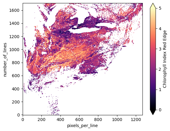
L2 PACE OCI data has multiple quality flags we could apply, but here we will only mask for CLDICE, the flag for pixels contaminated with clouds and/or ice. The names of each available flag and what they mean can be found at this link.
if vi_src["l2_flags"].cf.is_flag_variable:
    cloud_mask = ~(vi_src["l2_flags"].cf == "CLDICE")
    vi_src = vi_src.where(cloud_mask)
vi_src.cire.plot(cmap="magma", vmin=0, vmax=5)
plt.show()
Now that our dataset represents only (relatively) clear-sky pixels, we can move on to steps 2 - 4 of the reprojection, that is, assigning coordinates, spatial reference, and a CRS to the data. Note that this has to be done after the masking, as you will get an error in the reprojection step if the order is flipped.
vi_src.coords["longitude"] = vi_dt["navigation_data"]["longitude"]
vi_src.coords["latitude"] = vi_dt["navigation_data"]["latitude"]

vi_src = vi_src.rio.set_spatial_dims("pixels_per_line", "number_of_lines")
vi_src = vi_src.rio.write_crs("epsg:4326")
vi_src
<xarray.Dataset> Size: 122MB
Dimensions:      (number_of_lines: 1710, pixels_per_line: 1272)
Coordinates:
    longitude    (number_of_lines, pixels_per_line) float32 9MB ...
    latitude     (number_of_lines, pixels_per_line) float32 9MB ...
    spatial_ref  int64 8B 0
Dimensions without coordinates: number_of_lines, pixels_per_line
Data variables:
    ndvi         (number_of_lines, pixels_per_line) float32 9MB nan nan ... nan
    evi          (number_of_lines, pixels_per_line) float32 9MB nan nan ... nan
    ndwi         (number_of_lines, pixels_per_line) float32 9MB nan nan ... nan
    ndii         (number_of_lines, pixels_per_line) float32 9MB nan nan ... nan
    cci          (number_of_lines, pixels_per_line) float32 9MB nan nan ... nan
    ndsi         (number_of_lines, pixels_per_line) float32 9MB nan nan ... nan
    pri          (number_of_lines, pixels_per_line) float32 9MB nan nan ... nan
    cire         (number_of_lines, pixels_per_line) float32 9MB nan nan ... nan
    car          (number_of_lines, pixels_per_line) float32 9MB nan nan ... nan
    mari         (number_of_lines, pixels_per_line) float32 9MB nan nan ... nan
l2_flags (number_of_lines, pixels_per_line) float64 17MB nan ... 1.07...If we compare vi_src before and after these steps, it looks like nothing much has changed. However, you can see that under Coordinates we now have longitude and latitude, as well as the spatial_ref variable, which contains the spatial reference information necessary to reproject the data.
In the next cell, we create a destination dataset, vi_dst, the projected version of the source dataset. The key parameter in this step is the src_geoloc_array, which is how we’re able to feed the function our coordinate arrays and get out a projected dataset.
In this example, we project into EPSG 4326, which might not be best for your project. An easy way to input your preferred CRS is rasterio’s CRS module. For example, if you knew the specific EPSG code you wanted to use (e.g., 32617), you would replace vi_src.rio.crs with rasterio.crs.CRS.from_epsg(32617). There are several other options to define your CRS as well - see here for more details.
vi_dst = vi_src.rio.reproject(
    dst_crs=vi_src.rio.crs,         # Replace with your own!
    src_geoloc_array=(
        vi_src.coords["longitude"],
        vi_src.coords["latitude"],
    ),
    nodata=np.nan,
    resampling=Resampling.nearest,
).rename({"x":"longitude", "y":"latitude"})
We can plot the data with a basemap to see that it was correctly georeferenced and reprojected. Note that the rio.reproject function defines its own resolution and alignment relative to the input file by default; if you would like to define a constant grid, simply add in the dst_transform argument with your defined Affine transform.
Also of note: the coordinate names “longitude” and “latitude” get converted to “x” and “y”, respectively, during the reprojection. This is a quirk of rioxarray and does not affect the projection or the export in Section 3. We rename the coordinates with .rename({"x":"longitude", "y":"latitude"}) at the end of the cell above to avoid confusion.
fig, ax = plt.subplots(figsize=(9, 5), subplot_kw={"projection": ccrs.PlateCarree()})
ax.gridlines(draw_labels={"left": "y", "bottom": "x"}, linewidth=0.25)
ax.coastlines(linewidth=0.5)
ax.add_feature(cartopy.feature.OCEAN, edgecolor="w", linewidth=0.01)
ax.add_feature(cartopy.feature.LAND, edgecolor="w", linewidth=0.01)
ax.add_feature(cartopy.feature.LAKES, edgecolor="w", linewidth=0.01)
vi_dst["cire"].plot(cmap="magma", vmin=0, vmax=5)
plt.title("")
plt.show()
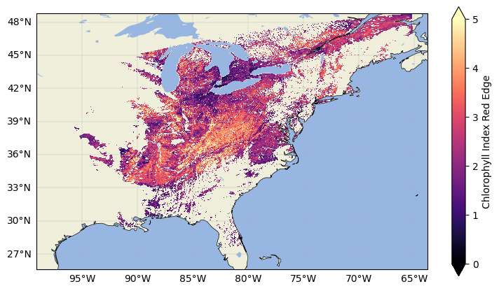
The VI data is now masked and reprojected! Now let’s start with our 3D surface reflectances.
2.2. 3D Variables - Surface Reflectance#
Typically, you’d be able to repeat the process we completed for the VIs above for most 3D data, and if you tried it with PACE OCI surface reflectances, it would work. However, in addition to reprojecting PACE OCI data, another goal of this tutorial is to export the data into GeoTIFF format for use in a GIS software. Many of these programs, and specifically the popular QGIS software, require that data dimensions are ordered (Z, Y, X), where Y and X are positional coordinates like latitude and longitude and Z is a third dimension, like wavelength.
Recalling from above, the surface reflectance variable rhos has 3 dimensions (rows, columns, wavelengths) - in other words, (Y, X, Z). Without resolving this issue, trying to load PACE OCI surface reflectance data in QGIS will result in what looks like nonsensical lines and squares instead of a rich reflectance data cube.
To put PACE OCI reflectances in the correct dimensional order, all we have to do is transpose the data so that the wavelength dimension, wavelength_3d, is first.
Before this, we include code that assigns the wavelength_3d variable as a coordinate, so that each band can be selected by its center wavelength rather than its 0-121 numerical index ordering.
sr_dt["geophysical_data"] = (
    sr_dt["geophysical_data"]
    .to_dataset()
    .assign_coords(sr_dt["sensor_band_parameters"].coords)
)
sr_dt["geophysical_data"]
<xarray.DatasetView> Size: 1GB
Dimensions:        (number_of_lines: 1710, pixels_per_line: 1272,
                    wavelength_3d: 122)
Coordinates:
  * wavelength_3d  (wavelength_3d) float64 976B 346.0 351.0 ... 2.258e+03
Dimensions without coordinates: number_of_lines, pixels_per_line
Data variables:
    rhos           (number_of_lines, pixels_per_line, wavelength_3d) float32 1GB ...
l2_flags (number_of_lines, pixels_per_line) int32 9MB ...sr_src = sr_dt["geophysical_data"]["rhos"]
sr_src = sr_src.transpose("wavelength_3d", ...)
sr_src
<xarray.DataArray 'rhos' (wavelength_3d: 122, number_of_lines: 1710,
                          pixels_per_line: 1272)> Size: 1GB
[265364640 values with dtype=float32]
Coordinates:
  * wavelength_3d  (wavelength_3d) float64 976B 346.0 351.0 ... 2.258e+03
Dimensions without coordinates: number_of_lines, pixels_per_line
Attributes:
    long_name:  Surface reflectance
    valid_min:  -0.05
valid_max: 1.0The rhos variable is now in dimension order (Z, Y, X), which will allow QGIS and other software with the same requirement to properly handle the surface reflectance data. Note that we are setting sr_src to include only rhos and not l2_flags. We separate these variables to allow for exporting in Section 3, as the rio.to_raster method cannot handle two dataarrays with different dimensions (i.e., 3D for rhos and 2D for l2_flags). That means if you want your surface reflectance data masked with any of the flags we explained above, you’ll have to do it before the step above.
We can now complete the rest of the steps above to reproject the data.
sr_src.coords["longitude"] = sr_dt["navigation_data"]["longitude"]
sr_src.coords["latitude"] = sr_dt["navigation_data"]["latitude"]

sr_src = sr_src.rio.set_spatial_dims("pixels_per_line", "number_of_lines")
sr_src = sr_src.rio.write_crs("epsg:4326")

sr_dst = sr_src.rio.reproject(
    dst_crs=sr_src.rio.crs,
    src_geoloc_array=(
        sr_src.coords["longitude"],
        sr_src.coords["latitude"],
    ),
    nodata=np.nan,
    resampling=Resampling.nearest,
).rename({"x":"longitude", "y":"latitude"})
fig, ax = plt.subplots(figsize=(9, 5), subplot_kw={"projection": ccrs.PlateCarree()})
ax.gridlines(draw_labels={"left": "y", "bottom": "x"}, linewidth=0.25)
ax.coastlines(linewidth=0.5)
ax.add_feature(cartopy.feature.OCEAN, edgecolor="w", linewidth=0.01)
ax.add_feature(cartopy.feature.LAND, edgecolor="w", linewidth=0.01)
ax.add_feature(cartopy.feature.LAKES, edgecolor="w", linewidth=0.01)
sr_dst.sel({"wavelength_3d": 860}).plot(cmap="Greys_r", vmin=0, vmax=1, zorder=101)
plt.title("")
plt.show()
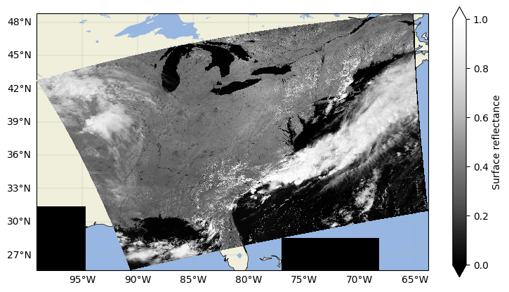
3. Exporting to GeoTIFF#
Now that we have two georeferenced, projected datasets of surface reflectances and VIs, you can export them to your preferred format. Here, we export to a Cloud Optimized Geotiff, or COG, using the “COG” driver with applicable profile options.
COGs are a subset of Geotiffs which have been optimized to work in cloud environments. If you are not working in the cloud, you don’t have to worry, as COGs are backwards compatible with Geotiffs. That is, any software that can be used to analyze a Geotiff can also be used with COGs. For more information on the COG format, please see the cogeo website. There is also a very useful plug in for rasterio called rio-cogeo for creating/validating COGs, documentation for which can be found here.
We create our files by building a profile from the destination datasets (sr_dst or vi_dst) and using the rio.to_raster() method. Each of the profile options is necessary for the format conversion, but can be changed to user preference as needed. For example, if you prefer a different nodata value, substitute the values you’d like to change in the dictionaries below.
sr_dst_name = Path(sr_path).with_suffix(".tif")
profile = {
    "driver": "COG",
    "width": sr_dst.shape[2],
    "height": sr_dst.shape[1],
    "count": sr_dst.shape[0],
    "crs": sr_dst.rio.crs,
    "dtype": sr_dst.dtype,
    "transform": sr_dst.rio.transform(),
    "compress": "lzw",
    "nodata": np.nan,
    "interleave":"BAND",
    "tiled":"YES",
    "blockxsize": "512", "blockysize": "512",
}
sr_dst.rio.to_raster(sr_dst_name, **profile)

vi_dst_name = Path(vi_path).with_suffix(".tif")
profile = {
    "driver": "COG",
    "width": vi_dst["cire"].shape[1],
    "height": vi_dst["cire"].shape[0],
    "count": 11,
    "crs": vi_dst.rio.crs,
    "dtype": vi_dst["cire"].dtype,
    "transform": vi_dst.rio.transform(),
    "compress": "lzw",
    "nodata": np.nan,
    "interleave":"BAND",
    "tiled":"YES",
    "blockxsize": "512", "blockysize": "512",
}
vi_dst.rio.to_raster(vi_dst_name, **profile)
The files should be successfully converted, and able to be analyzed properly in QGIS and other software! To make a nice quick true colour image in your program of choice, you can set R = 655 nm (band 60), G = 555 nm (band 42), and B = 470 nm (band 25).
To do the format conversion and reprojection in one step, please see the function below:
def nc_to_gtiff(fpath):
    """
    Convert a PACE SFREFL or LANDVI NetCDF file to GeoTIFF format
    Masks LANDVI dataset for clouds automatically
    Args:
        fpath - Path to NetCDF file to convert
    """
    dt = xr.open_datatree(fpath)
    fpath_s = str(fpath)

    if "SFREFL" in fpath_s:
        src = dt["geophysical_data"]["rhos"].transpose("wavelength_3d", ...)
    elif "LANDVI" in fpath_s:
        src = dt["geophysical_data"].to_dataset()
        if src["l2_flags"].cf.is_flag_variable:
            cloud_mask = ~(src["l2_flags"].cf == "CLDICE")
            src = src.where(cloud_mask)
    else:
        print(
            "File is neither the SFREFL nor LANDVI PACE suite, you'll have to adapt these methods yourself!"
        )
        return

    src.coords["longitude"] = dt["navigation_data"]["longitude"]
    src.coords["latitude"] = dt["navigation_data"]["latitude"]
    src = src.rio.set_spatial_dims("pixels_per_line", "number_of_lines")
    src = src.rio.write_crs("epsg:4326")

    dst = src.rio.reproject(
        dst_crs=src.rio.crs,
        src_geoloc_array=(src.coords["longitude"], src.coords["latitude"]),
        nodata=np.nan,
        resampling=Resampling.nearest,
    )

    if "SFREFL" in fpath_s:
        width, height, count = dst.shape[2], dst.shape[1], dst.shape[0]
        dtype = dst.dtype
    elif "LANDVI" in fpath_s:
        width, height, count = dst["cire"].shape[1], dst["cire"].shape[0], 11
        dtype = dst["cire"].dtype

    dst_name = Path(fpath).with_suffix(".tif")
    profile = {
        "driver": "COG",
        "width": width,
        "height": height,
        "count": count,
        "crs": dst.rio.crs,
        "dtype": dtype,
        "transform": dst.rio.transform(),
        "compress": "lzw",
        "nodata": np.nan,
        "interleave":"BAND",
        "tiled":"YES",
        "blockxsize": "512", "blockysize": "512",
    }

    dst.rio.to_raster(dst_name, **profile)
nc_to_gtiff(vi_path)
4. Converting Level-3 Data to GeoTIFF#
Level-3 Mapped (L3M) data is already mapped to a Plate Carrée projection–in other words, unless you want the data in another projection, you don’t need to reproject as we did for the L2 data above. In order to convert these files from NetCDF to GeoTIFF, all you need is to transpose the datasets as necessary and assign a CRS.
First, let’s download a Level-3 Global Mapped Surface Reflectance file.
results = earthaccess.search_data(
    short_name="PACE_OCI_L3M_LANDVI",
    granule_name="PACE_OCI.20240601_20240630.L3m.MO.LANDVI.V3_0.0p1deg.nc",
)
paths = earthaccess.download(results, local_path="data")
if "SFREFL" in str(paths[0]):
    ds = xr.open_dataset(paths[0]).rhos.transpose("wavelength", ...)
elif "LANDVI" in str(paths[0]):
    ds = xr.open_dataset(paths[0]).drop_vars("palette")

ds = ds.rio.write_crs("epsg:4326")
ds.rio.to_raster(Path(paths[0]).with_suffix(".tif"), driver="COG")
You have completed the notebook on reprojecting and format conversion of PACE OCI L2 data. We suggest looking at the notebook on “Machine Learning with Satellite Data” to explore some more advanced analysis methods.