
Applying L-S Periodogram Analysis to Ocean Color Data#
Authors: Riley Blocker (NASA, SSAI)
The following are prerequisites for this tutorial
A NASA Ocean Color Validation Data .csv file, which can also be downloaded from: https://seabass.gsfc.nasa.gov/search#val
Summary#
This notebook follows the astropy documentation for timeseries analysis to generate a Lomb-Scargle periodograms for Ocean Color (OC) data.
Learning Objectives#
At the end of this notebook you will know how to:
Generate a Lomb-Scargle periodogram for ocean color data time series
Calculate the False-Alarm-Probability to estimate the significance of a peak in the periodogram
Contents#
1. Setup#
import matplotlib as mpl
import matplotlib.pyplot as plt
import numpy as np
import pandas as pd
from astropy import units as u
from astropy.timeseries import LombScargle, TimeSeries

mpl.rcParams["lines.markersize"] = 5
mpl.rcParams["scatter.marker"] = "."
2. Validation Data#
NASA Ocean Color Validation Data can be extracted from https://seabass.gsfc.nasa.gov/search#val.
This example uses MOBY validation data paired with MODIS-Aqua measurements called “ModisA_Moby.csv” and saved within the “shared-public” directory.
To begin, we load the validation data as pandas dataframe and set the index to datetime.
df = pd.read_csv(
    "~/shared-public/pace-hackweek/modis_lombscargle_periodogram/ModisA_Moby.csv",
    header=33,
    skiprows=(35, 34),
)
df["date_time"] = pd.to_datetime(
    df["date_time"],
    format="%Y-%m-%d %H:%M:%S",
)
df = df.set_index("date_time")
We’re intersted in a metric evaluating the satellite-to-in situ matchup performance, so we add a \(\Delta R_{rs}(\lambda)\) column for the difference between the satellite and in situ observations.
df["Delta_rrs412"] = df["aqua_rrs412"] - df["insitu_rrs412"]
Convert the pandas data frame to an astropy time series.
ts = TimeSeries.from_pandas(df)
Plot MODIS-Aqua solar zenith angle versus time.
fig, ax = plt.subplots(figsize=(10, 3))

ax.scatter(ts.time.decimalyear, ts["aqua_solz"])
ax.set_xlabel("Year")
ax.set_ylabel(r"Degrees")
ax.set_title("Solar Zenith Angle")

plt.show()
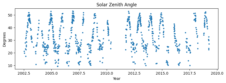
A regular annual variation clearly exists - as we’d expect given that Earth’s position along its orbit combined with its tilt along it’s own axis. But what about time series of a variable when there’s no prior knowledge of a regular temporal dependence or when noise may obscure the periodicity?
Plot \(\Delta\ R_{rs}(\lambda)\), Modis-Aqua \(R_{rs}(\lambda)\), and MOBY \(R_{rs}(\lambda)\) versus time
fig, axs = plt.subplots(3, 1, figsize=(10, 6), sharex=True)
year = ts.time.decimalyear

axs[0].scatter(year, ts["Delta_rrs412"])
axs[0].set_ylabel(r"$\Delta\ R_{rs}(412\ \mathrm{nm})$")
axs[0].set_title(r"MODIS-Aqua - MOBY")
axs[1].scatter(year, ts["insitu_rrs412"])
axs[1].set_ylabel(r"$R_{rs}(412\ \mathrm{nm})$")
axs[1].set_title(r"MOBY")
axs[2].scatter(year, ts["aqua_rrs412"])
axs[2].set_ylabel(r"$R_{rs}(412\ \mathrm{nm})$")
axs[2].set_title(r"MODIS-Aqua")
axs[2].set_xlabel("Year")

fig.tight_layout()
fig.show()
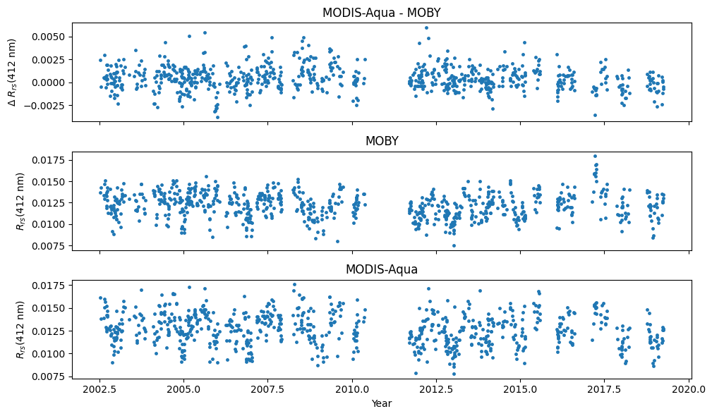
Unlike the solar zenith angle versus time (and to a lesser extent the \(R_{rs}(\lambda)\) time series), a periodicity in the \(\Delta R_{rs}(\lambda)\) time series is difficult to determine from the scatter plot.
3. Lomb-Scargle Periodogram#
A useful tool for detecting a periodicity in a discretely sampled signal is the periodogram. However, direct application of Fourier analysis techniques to generate a periodogram requires regular sampling, which is not always attainable in oceanographic data collection due to data gaps due to quality screening or instrument failures. Alternatively, a modified version of the periodogram - the Lomb-Scargle periodgram (or L-S periodgram) - can be achieved in connection to a least-squares analysis (VanderPlas, 2018) .
Generate Lomb-Scargle periodogram from the time series data. Specify parameters to use in the periodogram generation (see https://docs.astropy.org/en/stable/timeseries/lombscargle.html for descriptions).
ls_kwargs = {
    "nterms": 1,
    "normalization": "standard",
}
power_kwargs = {
    "minimum_frequency": 1 / (365.25 * 2.5) * (1 / u.day),
    "maximum_frequency": 1 / (7) * (1 / u.day),
    "samples_per_peak": 50,
    "method": "cython",
}
Generate and then plot the L-S periodogram.
ls = LombScargle.from_timeseries(ts, "aqua_solz", **ls_kwargs)
frequency, power = ls.autopower(**power_kwargs)
period = (1 / frequency).to("year")
fig, ax = plt.subplots(figsize=(4, 3))

ax.plot(period, power)
ax.set_title("Solar Zenith Angle")
ax.set_xlabel("Period [yr]")
ax.set_ylabel("Power")

fig.show()
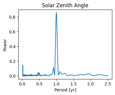
The estimated power in the L-S periodogram is dimensionless and ranges from 0 to 1. A peak’s height indicates that frequency of oscillation may exist in the signal, with increased likelihood with increased height. Here, we see a strong peak at a period of 1 year.
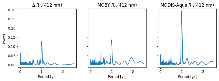
Generate Perdiograms for \(R_{rs}(\lambda)\)
uncertainty = ts["Delta_rrs412"].std()
DeltaRrs412_ls = LombScargle.from_timeseries(
    ts, "Delta_rrs412", uncertainty, **ls_kwargs
)
frequency, DeltaRrs412_power = DeltaRrs412_ls.autopower(**power_kwargs)
MobyRrs412_ls = LombScargle.from_timeseries(
    ts, "insitu_rrs412", 0.5 * uncertainty, **ls_kwargs
)
frequency, MobyRrs412_power = MobyRrs412_ls.autopower(**power_kwargs)
AquaRrs412_ls = LombScargle.from_timeseries(
    ts, "aqua_rrs412", 0.5 * uncertainty, **ls_kwargs
)
frequency, AquaRrs412_power = AquaRrs412_ls.autopower(**power_kwargs)
fig, axs = plt.subplots(1, 3, figsize=(10, 3), sharex=True, sharey=True)

axs[0].plot(period, DeltaRrs412_power)
axs[0].set_xlabel("Period [yr]")
axs[0].set_ylabel("Power")
axs[0].set_title(r"$\Delta\ R_{rs}(412\ \mathrm{nm})$")

axs[1].plot(period, MobyRrs412_power)
axs[1].set_xlabel("Period [yr]")
axs[1].set_title(r"MOBY $R_{rs}(412\ \mathrm{nm})$")

axs[2].plot(period, AquaRrs412_power)
axs[2].set_xlabel("Period [yr]")
axs[2].set_title(r"MODIS-Aqua $R_{rs}(412\ \mathrm{nm})$")

fig.show()
Find the “best” periodicity based on the maximum power.
period = period.round(3)
best_DeltaRrs412_period = period[np.argmax(DeltaRrs412_power)]
best_MobyRrs412_period = period[np.argmax(MobyRrs412_power)]
best_AquaRrs412_period = period[np.argmax(AquaRrs412_power)]
table = pd.DataFrame(
    index=[
        r"$\Delta R_{rs}(\lambda)$",
        r"MOBY $R_{rs}(\lambda)$",
        r"MODIS-Aqua  $R_{rs}(\lambda)$",
    ],
    data={
        "best_period": [
            best_DeltaRrs412_period,
            best_MobyRrs412_period,
            best_AquaRrs412_period,
        ]
    },
)
table[["best_period"]]
| best_period | |
|---|---|
| $\Delta R_{rs}(\lambda)$ | 1.005 yr |
| MOBY $R_{rs}(\lambda)$ | 0.995 yr |
| MODIS-Aqua $R_{rs}(\lambda)$ | 0.998 yr |
The “best” periods are all close to the annual period, which is within the precision uncertainity when the width of the peaks are considered.
4. False Alarm Probability#
A more useful metric for computing the uncertainty associated with the peak is the false alarm probablity (FAP) - a metric of how likely a peak’s height is due to coincidental alignment from noise instead of a true periodicity in the signal.
To find the FAP for the annual period, we get the position of the period closest to the annual period.
i = np.argmin(np.abs(period - 1 * u.year))
annual_power = DeltaRrs412_power[i]
DeltaRrs412_fap = DeltaRrs412_ls.false_alarm_probability(
    annual_power, method="bootstrap"
)
annual_power = MobyRrs412_power[i]
MobyRrs412_fap = MobyRrs412_ls.false_alarm_probability(annual_power, method="bootstrap")
annual_power = AquaRrs412_power[i]
AquaRrs412_fap = AquaRrs412_ls.false_alarm_probability(annual_power, method="bootstrap")
table["FAP"] = [
    DeltaRrs412_fap,
    MobyRrs412_fap,
    AquaRrs412_fap,
]
table[["FAP"]]
| FAP | |
|---|---|
| $\Delta R_{rs}(\lambda)$ | 0.0 |
| MOBY $R_{rs}(\lambda)$ | 0.0 |
| MODIS-Aqua $R_{rs}(\lambda)$ | 0.0 |
The FAPs at the annual period for for all the time series are zero, strongly indicating that the annual frequency is contained in the time series.
5. Folding the Time Series#
Now that we know with confidence that the annual peridicity is contained in the time series, we fold the temporal range to the annual peridocity. A day in the middle of the year is chosen so that the x-axis begins with Jan 1st (-182.56 days) and ends with Dec 31st (182.5).
folded_ts = ts.fold(period=1 * u.year, epoch_time="2000-07-02")
fig, axs = plt.subplots(1, 3, figsize=(10, 6), sharex=True, sharey=True)

x = folded_ts.time.jd
y = folded_ts["Delta_rrs412"]
axs[0].scatter(x, y)
axs[0].set_ylabel(r"$\Delta\ R_{rs}(412\ \mathrm{nm})$")
axs[0].set_title(r"MODIS-Aqua - MOBY")
axs[0].axhline(y=0, color="black", linewidth=2)

y = folded_ts["insitu_rrs412"]
axs[1].scatter(x, y)
axs[1].set_xlabel("Day of Year [day]")
axs[1].set_ylabel(r"$R_{rs}(412\ \mathrm{nm})$")
axs[1].set_title(r"MOBY")
axs[1].axhline(y=y.mean(), color="black", linewidth=2)

y = folded_ts["aqua_rrs412"]
axs[2].scatter(x, y)
axs[2].set_ylabel(r"$R_{rs}(412\ \mathrm{nm})$")
axs[2].set_title(r"MODIS-Aqua")
axs[2].axhline(y=y.mean(), color="black", linewidth=2)

fig.tight_layout()
fig.show()
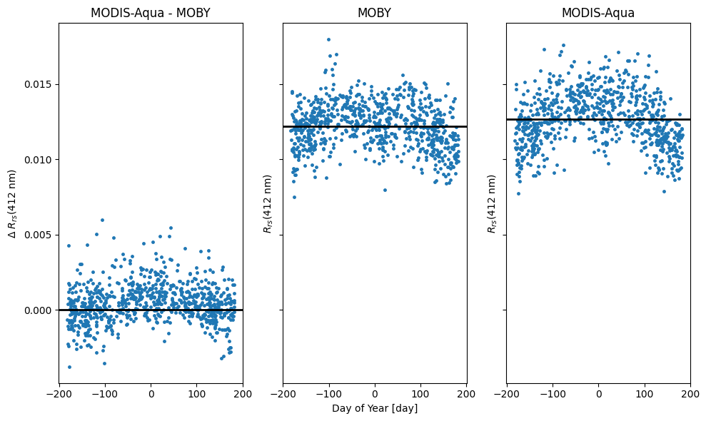
When folded, the annual perodicity is clearly contained in the time series (higher in the summer and lower in the winter).