
Visualize HARP2 CLOUD GPC Product#
Authors: Chamara (NASA, SSAI), Kirk (NASA), Andy (NASA, UMBC), Meng (NASA, SSAI), Sean (NASA, MSU)
Summary#
This notebook summarizes how to access HARP2 GISS Polarimetric Cloud (GPC) products (CLOUD_GPC.V3_0). Note that this notebook is based on an early preliminary version of the product and is therefore subject to future optimizations and changes.
Learning Objectives#
By the end of this notebook, you will understand:
How to acquire HARP2 L2 data
Available variables in the product
How to visualize variables
Contents#
1. Setup#
Begin by importing all of the packages used in this notebook. If your kernel uses an environment defined following the guidance on the tutorials page, then the imports will be successful.
from pathlib import Path
from textwrap import wrap

import cartopy.crs as ccrs
import earthaccess
import matplotlib.colors as mcolors
import matplotlib.pyplot as plt
import numpy as np
import requests
import xarray as xr

plt.style.use("seaborn-v0_8-notebook")
auth = earthaccess.login(persist=True)
fs = earthaccess.get_fsspec_https_session()
2. Get Level-2 Data#
HARP2 L2.CLOUD_GPC_NRT products are currently available starting from 2025-07-01. You can use the following “short name” to search with earthaccess.search_data:
results = earthaccess.search_datasets(instrument="harp2")
for item in results:
    summary = item.summary()
    print(summary["short-name"])
PACE_HARP2_L0_D1
PACE_HARP2_L0_D2
PACE_HARP2_L0_D3
PACE_HARP2_L1A_SCI
PACE_HARP2_L1B_SCI
PACE_HARP2_L1C_SCI
PACE_HARP2_L2_CLOUD_GPC
PACE_HARP2_L2_CLOUD_GPC_NRT
PACE_HARP2_L3M_CLOUD_GPC_NRT
results = earthaccess.search_data(
    short_name="PACE_HARP2_L2_CLOUD_GPC_NRT",
    temporal=("2025-07-02", "2025-07-02"),
    bounding_box=(-90, -15, -89, -14),  # (west, south, east, north) if desired
    count=1,
)
paths = earthaccess.open(results)
paths
[<File-like object S3FileSystem, ob-cumulus-prod-public/PACE_HARP2.20250702T183825.L2.CLOUD_GPC.V3_0.NRT.nc>]
datatree = xr.open_datatree(paths[0])
# datatree
Here we merge all the data group together for convenience in data manipulations.
dataset = xr.merge(datatree.to_dict().values())
# dataset
3. Understanding HARP2 L2.CLOUD_GPC Product Structure#
HARP2 CLOUD_GPC products provide descriptive metadata for the variables. However, given the early stage of the product, improvements and changes are expected in future versions.
def print_variable_description(datatree, ret_type_list, exclude=False):
    """
    To print variables and descriptions in a table
    """
    print(f"{'Variable':50} | {'Units':10} | Description")
    print("-" * 100)

    for var, da in datatree["geophysical_data"].items():
        # Check inclusion/exclusion logic
        match = any(key in var for key in ret_type_list)
        if (match and not exclude) or (not match and exclude):
            units = da.attrs.get("units", "")
            desc = da.attrs.get("long_name", "")
            wrapped = wrap(desc, 100)
            print(f"{var:50} | {units:10} | {wrapped[0]}")
            for line in wrapped[1:]:
                print(f"{'':50} | {'':10} | {line}")
Cloud Bow Retrievals#
One of the main retrieval techniques implemented is the parametric cloud bow retrieval method (Bréon & Goloub, 1998; Alexandrov et al., 2012). The phrase “cloud_bow” is appended to variable names, their corresponding diagnostic variables, and additional variables derived by combining them with OCI Level 2 products. For example, “cloud_bow_droplet_number_concentration_adiabatic” and “cloud_bow_liquid_water_path” are derived using the retrieved droplet size distributions along with OCI L2.CLOUD properties.
print_variable_description(datatree, ["bow"])
Variable                                           | Units      | Description
----------------------------------------------------------------------------------------------------
cloud_bow_droplet_effective_radius                 | um         | Cloud droplet effective radius obtained using Cloud Bow.  The bands used in the retrieval are (665).
cloud_bow_droplet_effective_radius_stddev          | um         | Standard deviation of cloud droplet effective radius obtained using Cloud Bow.
cloud_bow_droplet_effective_variance               | 1          | Cloud droplet effective variance obtained using Cloud Bow.  The bands used in the retrieval are
                                                   |            | (665).
cloud_bow_droplet_effective_variance_stddev        | 1          | Standard deviation of cloud droplet effective variance obtained using Cloud Bow.
cloud_bow_rms                                      | 1          | Root mean square of data fit to retrieved cloud droplet radius and variance obtained using Cloud
                                                   |            | Bow.
cloud_bow_fit_correlation                          | 1          | Correlation of data fit to retrieved cloud droplet radius and variance obtained using Cloud Bow.
cloud_bow_cirrus_correlation                       | 1          | Correlation of cirrus fit to retrieved cloud droplet radius and variance obtained using Cloud Bow.
cloud_bow_auxiliary_fit                            | 1          | Auxiliarly_fit parameters C, B, A, accounting for linear addition offset, Rayleigh term and P12
                                                   |            | scaling, respectively (Alexandrov et al., RSE 2012, Eq. 3). One set per wavelength used in fit.
cloud_bow_extinction_cross_section_355nm           | um2        | 355 nm extinction cross section based on 865 nm cloud bow effective radius and variance retrieval.
cloud_bow_extinction_cross_section_532nm           | um2        | 532 nm extinction cross section based on 865 nm cloud bow effective radius and variance retrieval.
cloud_bow_lidar_ratio_355nm                        | sr         | Ratio at 355 nm of extinction to backscatter at 180° scattering angle based on 865 nm cloud bow
                                                   |            | effective radius and variance retrieval.
cloud_bow_lidar_ratio_532nm                        | sr         | Ratio at 532 nm of extinction to backscatter at 180° scattering angle based on 865 nm cloud bow
                                                   |            | effective radius and variance retrieval.
cloud_bow_droplet_number_concentration_adiabatic   | # cm-3     | Cloud droplet number concentration assumes that the liquid water content is increasing with some
                                                   |            | assumed fraction of the adiabatic value. The assumptions and formulae used are summarized in
                                                   |            | Grosvenor et al. 2018 doi:10.1029/2017RG000593.
cloud_bow_liquid_water_path                        | g m-2      | Cloud liquid water path (LWP) is obtained from the product of optical thickness and droplet
                                                   |            | effective radius.  It is assumed that the liquid water content is increasing linearly with height
                                                   |            | from cloud base.
cloud_bow_quality_retrieval_fail                   | 1          | If no bits are set (=0), the results are concluded OK. If bits are set, there is an issue with the
                                                   |            | retrieval. Fill value is used when there is no cloud or no data to check for cloud.
RFT Retrievals#
The second retrieval technique is the Rainbow Fourier Transform (RFT) method (Alexandrov et al., 2012). The prefix cloud_rft is appended to variable names, their associated diagnostic variables, and other outputs generated by this algorithm.
print_variable_description(datatree, ["rft"])
Variable                                           | Units      | Description
----------------------------------------------------------------------------------------------------
cloud_rft_droplet_effective_radius_mode_0          | um         | Cloud droplet modes effective radius from RFT retrievals for mode 0.
cloud_rft_droplet_effective_radius_mode_1          | um         | Cloud droplet modes effective radius from RFT retrievals for mode 1.
cloud_rft_droplet_effective_variance_mode_0        | 1          | Cloud droplet modes effective variance from RFT retrievals for mode 0.
cloud_rft_droplet_effective_variance_mode_1        | 1          | Cloud droplet modes effective variance from RFT retrievals for mode 1.
cloud_rft_mode_fraction_0                          | 1          | Cloud droplet modes fraction from RFT retrievals for mode 0.
cloud_rft_mode_fraction_1                          | 1          | Cloud droplet modes fraction from RFT retrievals for mode 1.
cloud_rft_decomp_size_correlation                  | 1          | Correlation between the mode decomposition of the RFT and the size distribution.
cloud_rft_quality_retrieval_fail                   | 1          | If no bits are set (=0), the results are concluded OK. If bits are set, there is an issue with the
                                                   |            | retrieval. Fill value is used when there is no cloud or no data to check for cloud.
Cloud Liquid Index Retrievals#
print_variable_description(datatree, ["index"], exclude=False)
Variable                                           | Units      | Description
----------------------------------------------------------------------------------------------------
cloud_liquid_index                                 | 1          | Index indicating the strength of the primary rainbow in the observed polarized reflectances owing to
                                                   |            | scattering on liquid drops. A liquid index <0.3 is considered to exclude presence of liquid drops in
                                                   |            | the tops of the observed clouds, and thus indicates glaciated cloud tops (van Diedenhoven et al.,
                                                   |            | JAS 2012).
Additional Variables From OCI L2.CLOUD Products#
print_variable_description(datatree, ["index", "rft", "bow"], exclude=True)
Variable                                           | Units      | Description
----------------------------------------------------------------------------------------------------
cloud_top_altitude                                 | m          | Cloud top altitude
cloud_top_temperature                              | K          | Air temperature at the cloud top
cloud_top_pressure                                 | Pa         | Air pressure at the cloud top
cloud_optical_thickness                            | 1          | Cloud optical thickness obtained from AUX file.
cloud_quality                                      | 1          | If no bits are set (=0), the results are concluded OK. If bits are set, there is an issue with the
                                                   |            | retrieval. Fill value is used when there is no cloud or no data to check for cloud.
4. Visulizing Variables#
transform = ccrs.PlateCarree(central_longitude=0)
projection = ccrs.PlateCarree()


def extremes_removed_ids(x):
    """
    Returns indices of array x after removing the extreme values
    """
    q3 = np.percentile(x, 75)
    q1 = np.percentile(x, 25)
    xmin = q1 - 1.5 * (q3 - q1)
    xmax = q3 + 1.5 * (q3 - q1)
    return (xmin <= x) * (x < xmax)


def geo_axis_tags(ax, crs=ccrs.PlateCarree(central_longitude=0)):
    gl = ax.gridlines(crs=crs, draw_labels=True)
    ax.coastlines()
    # gl = ax.gridlines(draw_labels=True,linestyle='--',\
    #     xlocs=mticker.FixedLocator(np.arange(-180,180.1,10)),ylocs=mticker.FixedLocator(np.arange(-90,90.1,10)))
    gl.top_labels = False
    gl.right_labels = False
    gl.xlabel_style = {"size": 12, "color": "k"}
    gl.ylabel_style = {"size": 12, "color": "k"}

    ax.coastlines()
    return gl
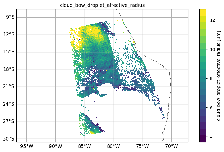
var = "cloud_bow_droplet_effective_radius"
fig1, ax1 = plt.subplots(figsize=(10, 6), subplot_kw={"projection": projection})
cmap = plt.get_cmap("viridis", 20)
_arr = dataset[var].values
arr_tes = np.ma.masked_array(_arr, mask=np.isnan(_arr))
# vmin, vmax = har_l2_tes.read_from_file('retrievals/%s'%variable_list[i],attrs_local='valid_min'), har_l2_tes.read_from_file('retrievals/%s'%variable_list[i],attrs_local='valid_max')
vmin, vmax = (
    arr_tes.compressed()[extremes_removed_ids(arr_tes.compressed())].min(),
    arr_tes.compressed()[extremes_removed_ids(arr_tes.compressed())].max(),
)
ctf = ax1.pcolormesh(
    dataset.longitude,
    dataset.latitude,
    arr_tes,
    transform=transform,
    cmap=cmap,
    vmin=vmin,
    vmax=vmax,
)
ax1.set_title(var, size=12)
gl = geo_axis_tags(ax1, crs=transform)
# plt.colorbar(pm, ax=ax_map, orientation="vertical", pad=0.1, label=label)
fig1.colorbar(
    ctf, ax=ax1, orientation="vertical", label="%s [%s]" % (var, dataset[var].units)
)
<matplotlib.colorbar.Colorbar at 0x7ffb09d15d10>
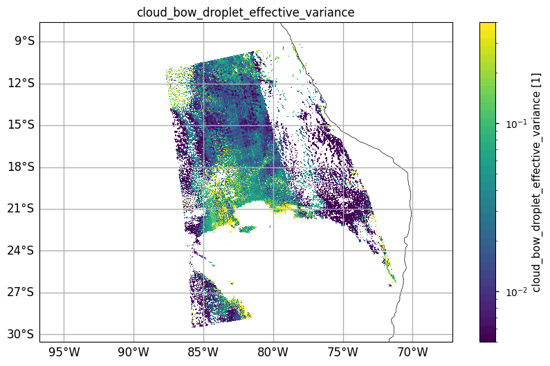
var = "cloud_bow_droplet_effective_variance"
fig1, ax1 = plt.subplots(figsize=(10, 6), subplot_kw={"projection": projection})
cmap = plt.get_cmap("viridis", 40)
norm = mcolors.LogNorm(vmin=0.005, vmax=0.4)
_arr = dataset[var].values
arr_tes = np.ma.masked_array(_arr, mask=np.isnan(_arr))
# vmin, vmax = arr_tes.compressed()[extremes_removed_ids(arr_tes.compressed())].min(), arr_tes.compressed()[extremes_removed_ids(arr_tes.compressed())].max()
ctf = ax1.pcolormesh(
    dataset.longitude,
    dataset.latitude,
    arr_tes,
    transform=transform,
    cmap=cmap,
    norm=norm,
)
ax1.set_title(var, size=12)
gl = geo_axis_tags(ax1, crs=transform)
# plt.colorbar(pm, ax=ax_map, orientation="vertical", pad=0.1, label=label)
fig1.colorbar(
    ctf, ax=ax1, orientation="vertical", label="%s [%s]" % (var, dataset[var].units)
)
<matplotlib.colorbar.Colorbar at 0x7ffb01237310>
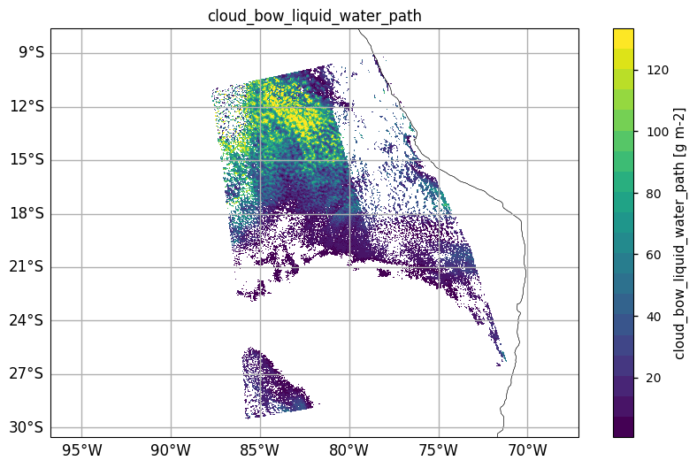
var = "cloud_bow_liquid_water_path"
fig1, ax1 = plt.subplots(figsize=(10, 6), subplot_kw={"projection": projection})
cmap = plt.get_cmap("viridis", 20)
_arr = dataset[var].values
arr_tes = np.ma.masked_array(_arr, mask=np.isnan(_arr))
# vmin, vmax = har_l2_tes.read_from_file('retrievals/%s'%variable_list[i],attrs_local='valid_min'), har_l2_tes.read_from_file('retrievals/%s'%variable_list[i],attrs_local='valid_max')
vmin, vmax = (
    arr_tes.compressed()[extremes_removed_ids(arr_tes.compressed())].min(),
    arr_tes.compressed()[extremes_removed_ids(arr_tes.compressed())].max(),
)
ctf = ax1.pcolormesh(
    dataset.longitude,
    dataset.latitude,
    arr_tes,
    transform=transform,
    cmap=cmap,
    vmin=vmin,
    vmax=vmax,
)
ax1.set_title(var, size=12)
gl = geo_axis_tags(ax1, crs=transform)
# plt.colorbar(pm, ax=ax_map, orientation="vertical", pad=0.1, label=label)
fig1.colorbar(
    ctf, ax=ax1, orientation="vertical", label="%s [%s]" % (var, dataset[var].units)
)
<matplotlib.colorbar.Colorbar at 0x7ffb0186f890>
5. Reference#
Breon, F.-M., & Doutriaux-Boucher, M. (2005). A comparison of cloud droplet radii measured from space. IEEE Transactions on Geoscience and Remote Sensing, 43(8), 1796–1805. https://doi.org/10.1109/TGRS.2005.852838
Alexandrov, M. D., Cairns, B., Emde, C., Ackerman, A. S., & Van Diedenhoven, B. (2012). Accuracy assessments of cloud droplet size retrievals from polarized reflectance measurements by the research scanning polarimeter. Remote Sensing of Environment, 125, 92–111. https://doi.org/10.1016/j.rse.2012.07.012
Van Diedenhoven, B., Fridlind, A. M., Ackerman, A. S., & Cairns, B. (2012). Evaluation of Hydrometeor Phase and Ice Properties in Cloud-Resolving Model Simulations of Tropical Deep Convection Using Radiance and Polarization Measurements. Journal of the Atmospheric Sciences, 69(11), 3290–3314. https://doi.org/10.1175/JAS-D-11-0314.1
Alexandrov, M. D., Cairns, B., & Mishchenko, M. I. (2012). Rainbow Fourier transform. Journal of Quantitative Spectroscopy and Radiative Transfer, 113(18), 2521–2535. https://doi.org/10.1016/j.jqsrt.2012.03.025