Parallel and Larger-than-Memory Processing

Authors: Ian Carroll (NASA, UMBC)

The following notebooks are prerequisites for this tutorial.

• Learn with OCI: Data Access

• Learn with OCI: Processing with Command-line Tools

• Learn with OCI: Project and Format

Summary

Processing a large collection of PACE granules can seem like a big job! The best way to approach a big data processing job is by breaking it into many small jobs, and then putting all the pieces back together again. The reason we break up big jobs has to do with computational resources, specifically memory (i.e. RAM) and processors (i.e. CPUs or GPUs). That large collection of granules can’t all fit in memory; and even if it could, your computation might only use one processor.

This notebook works toward a better understanding of a tool tightly integrated with XArray that breaks up big jobs. The tool is Dask: a Python library for parallel and distributed computing.

Learning Objectives

At the end of this notebook you will know:

• About the framework we’re calling “chunk-apply-combine”

• How to start a dask client for parallel and larger-than-memory pipelines

• One method for averaging Level-2 “swath” data over time

Contents

1. Setup

2. Chunk-Apply-Combine

3. Dask Workers

4. Level-2 Averaging

5. Scaling Out

1. Setup

Begin by importing all of the packages used in this notebook. If your kernel uses an environment defined following the guidance on the tutorials page, then the imports will be successful.

import cartopy.crs as ccrs
import dask.array as da
import earthaccess
import matplotlib.pyplot as plt
import numpy as np
import xarray as xr
from dask.distributed import Client
from matplotlib.patches import Rectangle

We will discuss dask in more detail below, but we use several additional packages behind-the-scenes. They are installed, but we don’t have to import them directly.

• rasterio is a high-level wrapper for GDAL which provides the ability to “warp” with the type of geolocation arrays distributed in Level-2 data.

• rioxarray is a wrapper that attaches the rasterio tools to XArray data structures

SatPy is another Python package that could be useful for the processing demonstrated in this notebok, especially through its Pyresample toolking. SatPy requires dedicated readers for any given instrument, however, and we have not tested the SatPy reader contributed for PACE/OCI.

The data used in the demonstration is the chlor_a product found in the BGC suite of Level-2 ocean color products from OCI.

bbox = (-77, 36, -73, 41)
results = earthaccess.search_data(
    short_name="PACE_OCI_L2_BGC",
    temporal=("2024-08-01", "2024-08-07"),
    bounding_box=bbox,
)
len(results)

16

The search results include all granules from launch through July of 2024 that intersect a bounding box around the Chesapeake and Delaware Bays. The region is much smaller than an OCI swath, so we do not use the cloud cover search filter which considers the whole swath.

results[0]

Data: PACE_OCI.20240801T174245.L2.OC_BGC.V3_0.nc

Size: 15.22 MB

Cloud Hosted: True

paths = earthaccess.open(results[:1])

datatree = xr.open_datatree(paths[0])

dataset = xr.merge(datatree.to_dict().values())
dataset = dataset.set_coords(("latitude", "longitude"))
chla = dataset["chlor_a"]
chla

<xarray.DataArray 'chlor_a' (number_of_lines: 1710, pixels_per_line: 1272)> Size: 9MB
[2175120 values with dtype=float32]
Coordinates:
    longitude  (number_of_lines, pixels_per_line) float32 9MB ...
    latitude   (number_of_lines, pixels_per_line) float32 9MB ...
Dimensions without coordinates: number_of_lines, pixels_per_line
Attributes:
    long_name:      Chlorophyll Concentration, OCI Algorithm
    units:          mg m^-3
    standard_name:  mass_concentration_of_chlorophyll_in_sea_water
    valid_min:      0.001
    valid_max:      100.0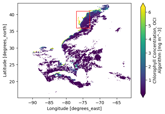
    reference:      Hu, C., Lee Z., and Franz, B.A. (2012). Chlorophyll-a alg...

xarray.DataArray

'chlor_a'

• number_of_lines: 1710
• pixels_per_line: 1272

• ...

  [2175120 values with dtype=float32]

• Coordinates: (2)
  • longitude
    (number_of_lines, pixels_per_line)
    float32
    ...

    long_name :

    Longitude

    units :

    degrees_east

    standard_name :

    longitude

    valid_min :

    -180.0

    valid_max :

    180.0

    [2175120 values with dtype=float32]

  • latitude
    (number_of_lines, pixels_per_line)
    float32
    ...

    long_name :

    Latitude

    units :

    degrees_north

    standard_name :

    latitude

    valid_min :

    -90.0

    valid_max :

    90.0

    [2175120 values with dtype=float32]

• Indexes: (0)
• Attributes: (6)

  long_name :

  Chlorophyll Concentration, OCI Algorithm

  units :

  mg m^-3

  standard_name :

  mass_concentration_of_chlorophyll_in_sea_water

  valid_min :

  0.001

  valid_max :

  100.0

  reference :

  Hu, C., Lee Z., and Franz, B.A. (2012). Chlorophyll-a algorithms for oligotrophic oceans: A novel approach based on three-band reflectance difference, J. Geophys. Res., 117, C01011, doi:10.1029/2011JC007395.

As a reminder, the Level-2 data has latitude and longitude arrays that give the geolocation of every pixel. The number_of_line and pixels_per_line dimensions don’t have any meaningful coordinates that would be useful for stacking Level-2 files over time. In a lot of the granules, like the one visualized here, there will be a tiny amount of data within the box. But we don’t want to lose a single pixel (if we can help it)!

fig = plt.figure(figsize=(8, 4))
axes = fig.add_subplot()
chla.plot.pcolormesh(x="longitude", y="latitude", robust=True, ax=axes)
axes.add_patch(
    Rectangle(
        bbox[:2],
        bbox[2] - bbox[0],
        bbox[3] - bbox[1],
        edgecolor="red",
        facecolor="none",
    )
)
axes.set_aspect("equal")
plt.show()

Here is where we first use rasterio and rioxarray. Those packages together add the rio attribute to the chla dataset which allows us to go GDAL processing in Python. GDAL requires certain metadata that rio records for us, but it needs to know some information! The Level-2 file uses the EPSG 4326 coordinate reference system, and the spatial dimensions are:

1. x (or longitude for EPSG 4326) is “pixels_per_line”

2. y (or latitude for EPSG 4326) is “number_of_lines”

chla = chla.rio.set_spatial_dims("pixels_per_line", "number_of_lines")
chla = chla.rio.write_crs("epsg:4326")

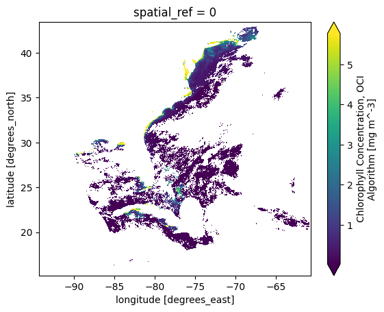
We can now use the reproject method to grid the L2 data into something like a Level-3 Mapped product, but for a single granule.

chla_L3M = chla.rio.reproject(
    dst_crs="epsg:4326",
    src_geoloc_array=(
        chla.coords["longitude"],
        chla.coords["latitude"],
    ),
)
chla_L3M = chla_L3M.rename({"x":"longitude", "y":"latitude"})

The plotting can now be done with imshow rather than pcolormesh.

plot = chla_L3M.plot.imshow(robust=True)

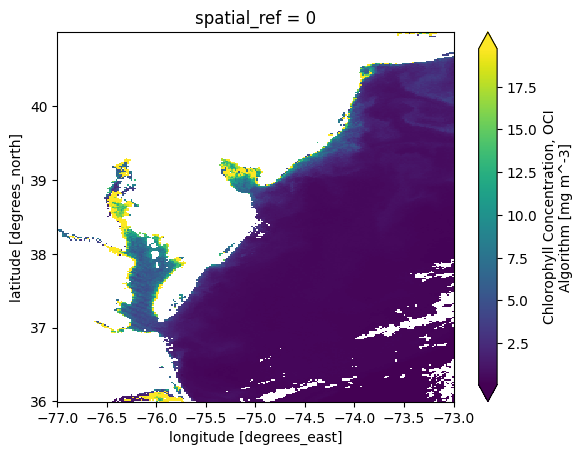
Also, we can easilly select the area-of-interest using our bounding box. This smaller data array will become our “template” for gridding additional granules below.

chla_L3M_aoi = chla_L3M.sel(
    {
        "longitude": slice(bbox[0], bbox[2]),
        "latitude": slice(bbox[3], bbox[1]),
    },
)
plot = chla_L3M_aoi.plot.imshow(robust=True)

When we get to opening mulitple datasets, we will use a helper function to create a “time” coordinate extracted from metadata.

def time_from_attr(ds):
    """Set the start time attribute as a dataset variable.

    Parameters
    ----------
    ds
        a dataset corresponding to a Level-2 granule
    """
    datetime = ds.attrs["time_coverage_start"].replace("Z", "")
    ds["time"] = ((), np.datetime64(datetime, "ns"))
    ds = ds.set_coords("time")
    return ds

Before we get to data, we will play with some random numbers. Whenever you use random numbers, a good practice is to set a fixed but unique seed, such as the result of secrets.randbits(64).

random = np.random.default_rng(seed=5179916885778238210)

back to top

3. Chunk-Apply-Combine

If you’ve done big data processing, you’ve probably come across the “split-apply-combine” or “map-reduce” frameworks. A simple case is computing group-wise means on a dataset where one variable defines the group and another variable is what you need to average for each group.

1. split: divide a table into smaller tables, one for each group

2. apply: calculte the mean on each small table

3. combine: reassemble the results into a table of group-wise means

The same framework is also used without a natural group by which a dataset should be divided. The split is on equal-sized slices of the original dataset, which we call “chunks”. Rather than a group-wise mean, you could use “chunk-apply-combine” to calculate the grand mean in chunks.

1. chunk: divide the array into smaller arrays, or “chunks”

2. apply: calculate the mean and sample size of each chunk (i.e. skipping missing values)

3. combine: combine the size-weighted means to compute the mean of the whole array

The apply and combine steps have to be capable of calculating results on a slice that can be combined to equal the result you would have gotten on the full array. If a computation can be shoved through “chunk-apply-combine” (see also “map-reduce”), then we can process an array that is too big to read into memory at once. We can also distribute the computation across processors or across a cluster of computers.

We can represent the framework visually using a task graph, a collection of functions (nodes) linked through input and output data (edges).

flowchart LR

A(random.normal) -->|array| B(mean)

The output of the random.normal function becomes the input to the mean function. We can decide to use chunk-apply-combine if either:

1. array is going to be larger than available memory

2. mean can be accurately calculated from intermediate results on slices of array

By the way, numpy arrays have an nbytes attribute that helps you understand how much memory you may need. Note tha most computations require several times the size of an input array to do the math.

array = random.normal(1, 2, size=2**24)
array

array([-2.21670758,  0.16399032,  2.69695432, ...,  0.95942182,
        0.46135808, -0.72953258], shape=(16777216,))

print(f"{array.nbytes / 2**20} MiB")

128.0 MiB

It’s still not too big to fit in memory on most laptops. For demonstration, let’s assume we could fit a 128 MiB array into memory, but not a 1 GiB array. We will calculate the mean of a 1 GiB array anyway, using 8 splits each of size 128 MiB in a serial pipeline.

A simple way to measure performance (i.e. speed) in notebooks is to use the IPython %%timeit magic. Begin any cell with %%timeit on a line by itself to trigger that cell to run many times under a timer. How long it takes the cell to run on average will be printed along with any result.

On this system, the serial approach can be seen below to take between 2 and 3 seconds.

%%timeit -r 3

n = 8
s = 0
for _ in range(n):
    array = random.normal(1, 2, size=2**24)
    s += array.mean()
mean = s / n

3.15 s ± 37.3 ms per loop (mean ± std. dev. of 3 runs, 1 loop each)

All we can implement in a for-loop is serial computation, but we have multiple processors available!

To help visualize the “chunk-apply-combine” framework, we can make a task graph for the “distributed” approach to calculating the mean of a very large array.

%%{ init: { 'flowchart': { 'curve': 'monotoneY' } } }%%

flowchart LR

A(random.normal)
A -->|array_0| C0(apply-mean)
A -->|array_1| C1(apply-mean)
A -->|array_2| C2(apply-mean)
subgraph cluster
C0
C1
C2
end
C0 -->|result_0| D(combine-mean)
C1 -->|result_1| D
C2 -->|result_2| D

In this task graph, the mean function is never used! Instead an apply-mean function and combine-mean functions are used to perform the appropriate computations on chunks and then combine the results to the global mean.

The two things that dask provides is the cluster that distributes jobs for computation as well as many functions (i.e. like apply-mean and combine-mean) that are the “chunk-apply-combine” equivalents of numpy functions.

To begin processing with dask, we start a local client to manage a cluster.

client = Client(n_workers=4, threads_per_worker=1, memory_limit="512MiB")
client

Client

Client-65dc4b21-7221-11f0-8863-86640707dd06

Connection method: Cluster object	Cluster type: distributed.LocalCluster
Dashboard: /user/itcarroll/proxy/8787/status

Launch dashboard in JupyterLab

Cluster Info

LocalCluster

bb7ddd98

Dashboard: /user/itcarroll/proxy/8787/status	Workers: 4
Total threads: 4	Total memory: 2.00 GiB
Status: running	Using processes: True

Scheduler Info

Scheduler

Scheduler-eb32c1a2-f381-41e4-a92f-ed70c94af3ba

Comm: tcp://127.0.0.1:42959	Workers: 0
Dashboard: /user/itcarroll/proxy/8787/status	Total threads: 0
Started: Just now	Total memory: 0 B

Workers

Worker: 0

Comm: tcp://127.0.0.1:38191	Total threads: 1
Dashboard: /user/itcarroll/proxy/34781/status	Memory: 512.00 MiB
Nanny: tcp://127.0.0.1:43369
Local directory: /tmp/dask-scratch-space/worker-j32driyx

Worker: 1

Comm: tcp://127.0.0.1:44573	Total threads: 1
Dashboard: /user/itcarroll/proxy/43543/status	Memory: 512.00 MiB
Nanny: tcp://127.0.0.1:43541
Local directory: /tmp/dask-scratch-space/worker-a1c69w_h

Worker: 2

Comm: tcp://127.0.0.1:46121	Total threads: 1
Dashboard: /user/itcarroll/proxy/33783/status	Memory: 512.00 MiB
Nanny: tcp://127.0.0.1:41171
Local directory: /tmp/dask-scratch-space/worker-refakx76

Worker: 3

Comm: tcp://127.0.0.1:43639	Total threads: 1
Dashboard: /user/itcarroll/proxy/34355/status	Memory: 512.00 MiB
Nanny: tcp://127.0.0.1:43673
Local directory: /tmp/dask-scratch-space/worker-_wra1s54

Just like np.random, we can use da.random from dask to generate a data array.

dask_random = da.random.default_rng(random)
dask_array = dask_random.normal(1, 2, size=2**27, chunks=2**22)
dask_array

Array Chunk Bytes 1.00 GiB 32.00 MiB Shape (134217728,) (4194304,) Dask graph 32 chunks in 1 graph layer Data type float64 numpy.ndarray

Apply the mean function with out dask_array is quite a bit different.

dask_array.mean()

Array Chunk Bytes 8 B 8 B Shape () () Dask graph 1 chunks in 5 graph layers Data type float64 numpy.ndarray

No operation has happened on the array. In fact, the random numbers have not even been generated yet! No resources are put into action until we explicitly demand a computation; for example, by calling compute, requesting a visualization, or writing data to disk.

%%timeit -r 3

mean = dask_array.mean().compute()

2.02 s ± 64.1 ms per loop (mean ± std. dev. of 3 runs, 1 loop each)

We just demonstrated two ways of doing larger-than-memory calculations.

Our synchronous implemenation (using a for loop) took the strategy of maximizing the use of available memory while processing one chunk: so we used 128 MiB chunks, requiring 8 chunks to get to a 1 GiB array.

Our concurrent implementation (using dask.array), took the strategy of maximizing the use of available processors: so we used small chunks of 32 MiB, requiring 32 to get to a 1 GiB array.

The concurrent implementation was about twice as fast, but your mileage may vary.

client.close()

4. Stacking Level-2 Granules

The integration of XArray and Dask is designed to let you work without doing much very differently. Of course, there is still a lot of work to do when writing any processing pipeline on a collection of Level-2 granules. Stacking them over time, for instance, may sound easy but requires resampling the data to a common grid.

This section demonstrates one method for stacking Level-2 granules. More details are available in the pre-requiste notebook noted above.

paths = earthaccess.open(results)

paths

[<File-like object S3FileSystem, ob-cumulus-prod-public/PACE_OCI.20240801T174245.L2.OC_BGC.V3_0.nc>,
 <File-like object S3FileSystem, ob-cumulus-prod-public/PACE_OCI.20240802T163900.L2.OC_BGC.V3_0.nc>,
 <File-like object S3FileSystem, ob-cumulus-prod-public/PACE_OCI.20240802T164400.L2.OC_BGC.V3_0.nc>,
 <File-like object S3FileSystem, ob-cumulus-prod-public/PACE_OCI.20240802T181718.L2.OC_BGC.V3_0.nc>,
 <File-like object S3FileSystem, ob-cumulus-prod-public/PACE_OCI.20240803T171333.L2.OC_BGC.V3_0.nc>,
 <File-like object S3FileSystem, ob-cumulus-prod-public/PACE_OCI.20240803T171833.L2.OC_BGC.V3_0.nc>,
 <File-like object S3FileSystem, ob-cumulus-prod-public/PACE_OCI.20240804T161447.L2.OC_BGC.V3_0.nc>,
 <File-like object S3FileSystem, ob-cumulus-prod-public/PACE_OCI.20240804T174805.L2.OC_BGC.V3_0.nc>,
 <File-like object S3FileSystem, ob-cumulus-prod-public/PACE_OCI.20240805T164420.L2.OC_BGC.V3_0.nc>,
 <File-like object S3FileSystem, ob-cumulus-prod-public/PACE_OCI.20240805T164920.L2.OC_BGC.V3_0.nc>,
 <File-like object S3FileSystem, ob-cumulus-prod-public/PACE_OCI.20240805T182239.L2.OC_BGC.V3_0.nc>,
 <File-like object S3FileSystem, ob-cumulus-prod-public/PACE_OCI.20240806T171853.L2.OC_BGC.V3_0.nc>,
 <File-like object S3FileSystem, ob-cumulus-prod-public/PACE_OCI.20240806T172353.L2.OC_BGC.V3_0.nc>,
 <File-like object S3FileSystem, ob-cumulus-prod-public/PACE_OCI.20240807T162007.L2.OC_BGC.V3_0.nc>,
 <File-like object S3FileSystem, ob-cumulus-prod-public/PACE_OCI.20240807T175325.L2.OC_BGC.V3_0.nc>,
 <File-like object S3FileSystem, ob-cumulus-prod-public/PACE_OCI.20240807T175825.L2.OC_BGC.V3_0.nc>]

kwargs = {"combine": "nested", "concat_dim": "time"}
attrs = xr.open_mfdataset(paths, preprocess=time_from_attr, **kwargs)
attrs

<xarray.Dataset> Size: 128B
Dimensions:  (time: 16)
Coordinates:
  * time     (time) datetime64[ns] 128B 2024-08-01T17:42:45.090000 ... 2024-0...
Data variables:
    *empty*
Attributes: (12/45)
    title:                             OCI Level-2 Data BGC
    product_name:                      PACE_OCI.20240801T174245.L2.OC_BGC.V3_...
    processing_version:                3.0
    history:                           l2gen par=/data1/sdpsoper/vdc/vpu0/wor...
    instrument:                        OCI
    platform:                          PACE
    ...                                ...
    geospatial_lon_max:                -60.75639
    geospatial_lon_min:                -94.36226
    startDirection:                    Ascending
    endDirection:                      Ascending
    day_night_flag:                    Day
    earth_sun_distance_correction:     0.970880389213562

xarray.Dataset

• Dimensions:
  • time: 16
• Coordinates: (1)
  • time
    (time)
    datetime64[ns]
    2024-08-01T17:42:45.090000 ... 2...

    array(['2024-08-01T17:42:45.090000000', '2024-08-02T16:39:00.164000000',
           '2024-08-02T16:44:00.222000000', '2024-08-02T18:17:18.145000000',
           '2024-08-03T17:13:33.220000000', '2024-08-03T17:18:33.103000000',
           '2024-08-04T16:14:47.125000000', '2024-08-04T17:48:05.224000000',
           '2024-08-05T16:44:20.124000000', '2024-08-05T16:49:20.182000000',
           '2024-08-05T18:22:39.158000000', '2024-08-06T17:18:53.181000000',
           '2024-08-06T17:23:53.063000000', '2024-08-07T16:20:07.086000000',
           '2024-08-07T17:53:25.185000000', '2024-08-07T17:58:25.067000000'],
          dtype='datetime64[ns]')

• Data variables: (0)
• Indexes: (1)
  • time
    PandasIndex

    PandasIndex(DatetimeIndex(['2024-08-01 17:42:45.090000', '2024-08-02 16:39:00.164000',
                   '2024-08-02 16:44:00.222000', '2024-08-02 18:17:18.145000',
                   '2024-08-03 17:13:33.220000', '2024-08-03 17:18:33.103000',
                   '2024-08-04 16:14:47.125000', '2024-08-04 17:48:05.224000',
                   '2024-08-05 16:44:20.124000', '2024-08-05 16:49:20.182000',
                   '2024-08-05 18:22:39.158000', '2024-08-06 17:18:53.181000',
                   '2024-08-06 17:23:53.063000', '2024-08-07 16:20:07.086000',
                   '2024-08-07 17:53:25.185000', '2024-08-07 17:58:25.067000'],
                  dtype='datetime64[ns]', name='time', freq=None))

• Attributes: (45)

  title :

  OCI Level-2 Data BGC

  product_name :

  PACE_OCI.20240801T174245.L2.OC_BGC.V3_0.nc

  processing_version :

  3.0

  history :

  l2gen par=/data1/sdpsoper/vdc/vpu0/workbuf/PACE_OCI.20240801T174245.L1B.V3.nc.param metafile=PACE_OCI.20240801T174245.L2.OC_BGC.V3_0.nc.meta

  instrument :

  OCI

  platform :

  PACE

  Conventions :

  CF-1.8, ACDD-1.3

  license :

  https://science.nasa.gov/earth-science/earth-science-data/data-information-policy/

  naming_authority :

  gov.nasa.gsfc.sci.oceandata

  id :

  3.0/L2/PACE_OCI.20240801T174245.L2.OC_BGC.V3_0.nc

  date_created :

  2025-02-11T07:42:34.000Z

  standard_name_vocabulary :

  CF Standard Name Table v36

  institution :

  NASA Goddard Space Flight Center, Ocean Ecology Laboratory, Ocean Biology Processing Group

  creator_name :

  NASA/GSFC/OBPG

  creator_email :

  data@oceancolor.gsfc.nasa.gov

  creator_url :

  https://oceandata.sci.gsfc.nasa.gov

  project :

  Ocean Biology Processing Group (NASA/GSFC/OBPG)

  publisher_name :

  NASA/GSFC/OBPG

  publisher_url :

  https://oceandata.sci.gsfc.nasa.gov

  publisher_email :

  data@oceancolor.gsfc.nasa.gov

  identifier_product_doi_authority :

  http://dx.doi.org

  identifier_product_doi :

  10.5067/PACE/OCI/L2/OC_BGC/3.0

  processing_level :

  L2

  cdm_data_type :

  swath

  spatialResolution :

  1000 m

  time_coverage_start :

  2024-08-01T17:42:45.090Z

  time_coverage_end :

  2024-08-01T17:47:44.972Z

  start_center_longitude :

  -73.43166

  start_center_latitude :

  18.61164

  end_center_longitude :

  -79.34041

  end_center_latitude :

  41.081535

  northernmost_latitude :

  43.41279

  southernmost_latitude :

  15.190758

  easternmost_longitude :

  -60.75639

  westernmost_longitude :

  -94.36226

  geospatial_lat_units :

  degrees_north

  geospatial_lon_units :

  degrees_east

  geospatial_lat_max :

  43.41279

  geospatial_lat_min :

  15.190758

  geospatial_lon_max :

  -60.75639

  geospatial_lon_min :

  -94.36226

  startDirection :

  Ascending

  endDirection :

  Ascending

  day_night_flag :

  Day

  earth_sun_distance_correction :

  0.970880389213562

Now, if you try xr.open_mfdataset you will probably encounter an error due to the fact that the number_of_lines is not the same in every granule.

products = xr.open_mfdataset(paths, group="geophysical_data", **kwargs)

---------------------------------------------------------------------------
AlignmentError                            Traceback (most recent call last)
Cell In[25], line 1
----> 1 products = xr.open_mfdataset(paths, group="geophysical_data", **kwargs)

File /srv/conda/envs/notebook/lib/python3.11/site-packages/xarray/backends/api.py:1706, in open_mfdataset(paths, chunks, concat_dim, compat, preprocess, engine, data_vars, coords, combine, parallel, join, attrs_file, combine_attrs, **kwargs)
   1702 try:
   1703     if combine == "nested":
   1704         # Combined nested list by successive concat and merge operations
   1705         # along each dimension, using structure given by "ids"
-> 1706         combined = _nested_combine(
   1707             datasets,
   1708             concat_dims=concat_dim,
   1709             compat=compat,
   1710             data_vars=data_vars,
   1711             coords=coords,
   1712             ids=ids,
   1713             join=join,
   1714             combine_attrs=combine_attrs,
   1715         )
   1716     elif combine == "by_coords":
   1717         # Redo ordering from coordinates, ignoring how they were ordered
   1718         # previously
   1719         combined = combine_by_coords(
   1720             datasets,
   1721             compat=compat,
   (...)
   1725             combine_attrs=combine_attrs,
   1726         )

File /srv/conda/envs/notebook/lib/python3.11/site-packages/xarray/structure/combine.py:367, in _nested_combine(datasets, concat_dims, compat, data_vars, coords, ids, fill_value, join, combine_attrs)
    364 _check_shape_tile_ids(combined_ids)
    366 # Apply series of concatenate or merge operations along each dimension
--> 367 combined = _combine_nd(
    368     combined_ids,
    369     concat_dims,
    370     compat=compat,
    371     data_vars=data_vars,
    372     coords=coords,
    373     fill_value=fill_value,
    374     join=join,
    375     combine_attrs=combine_attrs,
    376 )
    377 return combined

File /srv/conda/envs/notebook/lib/python3.11/site-packages/xarray/structure/combine.py:246, in _combine_nd(combined_ids, concat_dims, data_vars, coords, compat, fill_value, join, combine_attrs)
    242 # Each iteration of this loop reduces the length of the tile_ids tuples
    243 # by one. It always combines along the first dimension, removing the first
    244 # element of the tuple
    245 for concat_dim in concat_dims:
--> 246     combined_ids = _combine_all_along_first_dim(
    247         combined_ids,
    248         dim=concat_dim,
    249         data_vars=data_vars,
    250         coords=coords,
    251         compat=compat,
    252         fill_value=fill_value,
    253         join=join,
    254         combine_attrs=combine_attrs,
    255     )
    256 (combined_ds,) = combined_ids.values()
    257 return combined_ds

File /srv/conda/envs/notebook/lib/python3.11/site-packages/xarray/structure/combine.py:278, in _combine_all_along_first_dim(combined_ids, dim, data_vars, coords, compat, fill_value, join, combine_attrs)
    276     combined_ids = dict(sorted(group))
    277     datasets = combined_ids.values()
--> 278     new_combined_ids[new_id] = _combine_1d(
    279         datasets, dim, compat, data_vars, coords, fill_value, join, combine_attrs
    280     )
    281 return new_combined_ids

File /srv/conda/envs/notebook/lib/python3.11/site-packages/xarray/structure/combine.py:301, in _combine_1d(datasets, concat_dim, compat, data_vars, coords, fill_value, join, combine_attrs)
    299 if concat_dim is not None:
    300     try:
--> 301         combined = concat(
    302             datasets,
    303             dim=concat_dim,
    304             data_vars=data_vars,
    305             coords=coords,
    306             compat=compat,
    307             fill_value=fill_value,
    308             join=join,
    309             combine_attrs=combine_attrs,
    310         )
    311     except ValueError as err:
    312         if "encountered unexpected variable" in str(err):

File /srv/conda/envs/notebook/lib/python3.11/site-packages/xarray/structure/concat.py:277, in concat(objs, dim, data_vars, coords, compat, positions, fill_value, join, combine_attrs, create_index_for_new_dim)
    264     return _dataarray_concat(
    265         objs,
    266         dim=dim,
   (...)
    274         create_index_for_new_dim=create_index_for_new_dim,
    275     )
    276 elif isinstance(first_obj, Dataset):
--> 277     return _dataset_concat(
    278         objs,
    279         dim=dim,
    280         data_vars=data_vars,
    281         coords=coords,
    282         compat=compat,
    283         positions=positions,
    284         fill_value=fill_value,
    285         join=join,
    286         combine_attrs=combine_attrs,
    287         create_index_for_new_dim=create_index_for_new_dim,
    288     )
    289 else:
    290     raise TypeError(
    291         "can only concatenate xarray Dataset and DataArray "
    292         f"objects, got {type(first_obj)}"
    293     )

File /srv/conda/envs/notebook/lib/python3.11/site-packages/xarray/structure/concat.py:523, in _dataset_concat(datasets, dim, data_vars, coords, compat, positions, fill_value, join, combine_attrs, create_index_for_new_dim)
    520 # Make sure we're working on a copy (we'll be loading variables)
    521 datasets = [ds.copy() for ds in datasets]
    522 datasets = list(
--> 523     align(
    524         *datasets, join=join, copy=False, exclude=[dim_name], fill_value=fill_value
    525     )
    526 )
    528 dim_coords, dims_sizes, coord_names, data_names, vars_order = _parse_datasets(
    529     datasets
    530 )
    531 dim_names = set(dim_coords)

File /srv/conda/envs/notebook/lib/python3.11/site-packages/xarray/structure/alignment.py:944, in align(join, copy, indexes, exclude, fill_value, *objects)
    748 """
    749 Given any number of Dataset and/or DataArray objects, returns new
    750 objects with aligned indexes and dimension sizes.
   (...)
    934 
    935 """
    936 aligner = Aligner(
    937     objects,
    938     join=join,
   (...)
    942     fill_value=fill_value,
    943 )
--> 944 aligner.align()
    945 return aligner.results

File /srv/conda/envs/notebook/lib/python3.11/site-packages/xarray/structure/alignment.py:637, in Aligner.align(self)
    635 self.find_matching_unindexed_dims()
    636 self.align_indexes()
--> 637 self.assert_unindexed_dim_sizes_equal()
    639 if self.join == "override":
    640     self.override_indexes()

File /srv/conda/envs/notebook/lib/python3.11/site-packages/xarray/structure/alignment.py:499, in Aligner.assert_unindexed_dim_sizes_equal(self)
    497     add_err_msg = ""
    498 if len(sizes) > 1:
--> 499     raise AlignmentError(
    500         f"cannot reindex or align along dimension {dim!r} "
    501         f"because of conflicting dimension sizes: {sizes!r}" + add_err_msg
    502     )

AlignmentError: cannot reindex or align along dimension 'number_of_lines' because of conflicting dimension sizes: {1709, 1710}

Even if they were consistent, each granule has a different array of coordinates for latitude and longitude. Before doing a calculation over time, we need to project the Level-2 arrays to a common grid. Here is a function to do the same kind of gridding as above, but allowing us to pass the “destination” (.i.e. dst) projection parameters.

def grid_match(path, dst_crs, dst_shape, dst_transform):
    """Reproject a Level-2 granule to match a Level-3M-ish granule."""
    dt = xr.open_datatree(path)
    da = dt["geophysical_data"]["chlor_a"]
    da = da.rio.set_spatial_dims("pixels_per_line", "number_of_lines")
    da = da.rio.set_crs("epsg:4326")
    da = da.rio.reproject(
        dst_crs,
        shape=dst_shape,
        transform=dst_transform,
        src_geoloc_array=(
            dt["navigation_data"]["longitude"],
            dt["navigation_data"]["latitude"],
        ),
    )
    da = da.rename({"x":"longitude", "y":"latitude"})
    return da

Let’s try out the function, using chla_L3M_aoi as our template.

crs = chla_L3M_aoi.rio.crs
shape = chla_L3M_aoi.rio.shape
transform = chla_L3M_aoi.rio.transform()

grid_match(paths[0], crs, shape, transform)

<xarray.DataArray 'chlor_a' (latitude: 296, longitude: 237)> Size: 281kB
array([[          nan,           nan,           nan, ...,           nan,
                  nan, 1.0616910e+02],
       [          nan,           nan,           nan, ...,           nan,
                  nan,           nan],
       [          nan,           nan,           nan, ...,           nan,
                  nan,           nan],
       ...,
       [          nan,           nan,           nan, ...,           nan,
                  nan, 6.8380810e-02],
       [          nan,           nan,           nan, ...,           nan,
                  nan, 6.6567786e-02],
       [          nan,           nan,           nan, ...,           nan,
                  nan, 6.5402456e-02]], shape=(296, 237), dtype=float32)
Coordinates:
  * longitude    (longitude) float64 2kB -76.99 -76.98 -76.96 ... -73.02 -73.01
  * latitude     (latitude) float64 2kB 40.99 40.97 40.96 ... 36.04 36.02 36.01
    spatial_ref  int64 8B 0
Attributes:
    long_name:      Chlorophyll Concentration, OCI Algorithm
    units:          mg m^-3
    standard_name:  mass_concentration_of_chlorophyll_in_sea_water
    valid_min:      0.001
    valid_max:      100.0
    reference:      Hu, C., Lee Z., and Franz, B.A. (2012). Chlorophyll-a alg...

xarray.DataArray

'chlor_a'

• latitude: 296
• longitude: 237

• nan nan nan nan nan nan nan ... 0.06594 0.06462 nan nan nan nan 0.0654

  array([[          nan,           nan,           nan, ...,           nan,
                    nan, 1.0616910e+02],
         [          nan,           nan,           nan, ...,           nan,
                    nan,           nan],
         [          nan,           nan,           nan, ...,           nan,
                    nan,           nan],
         ...,
         [          nan,           nan,           nan, ...,           nan,
                    nan, 6.8380810e-02],
         [          nan,           nan,           nan, ...,           nan,
                    nan, 6.6567786e-02],
         [          nan,           nan,           nan, ...,           nan,
                    nan, 6.5402456e-02]], shape=(296, 237), dtype=float32)

• Coordinates: (3)
  • longitude
    (longitude)
    float64
    -76.99 -76.98 ... -73.02 -73.01

    axis :

    X

    long_name :

    longitude

    standard_name :

    longitude

    units :

    degrees_east

    array([-76.992763, -76.975869, -76.958975, ..., -73.039583, -73.02269 ,
           -73.005796], shape=(237,))

  • latitude
    (latitude)
    float64
    40.99 40.97 40.96 ... 36.02 36.01

    axis :

    Y

    long_name :

    latitude

    standard_name :

    latitude

    units :

    degrees_north

    array([40.990906, 40.974012, 40.957118, ..., 36.040984, 36.02409 , 36.007197],
          shape=(296,))

  • spatial_ref
    ()
    int64
    0

    crs_wkt :

    GEOGCS["WGS 84",DATUM["WGS_1984",SPHEROID["WGS 84",6378137,298.257223563,AUTHORITY["EPSG","7030"]],AUTHORITY["EPSG","6326"]],PRIMEM["Greenwich",0,AUTHORITY["EPSG","8901"]],UNIT["degree",0.0174532925199433,AUTHORITY["EPSG","9122"]],AXIS["Latitude",NORTH],AXIS["Longitude",EAST],AUTHORITY["EPSG","4326"]]

    semi_major_axis :

    6378137.0

    semi_minor_axis :

    6356752.314245179

    inverse_flattening :

    298.257223563

    reference_ellipsoid_name :

    WGS 84

    longitude_of_prime_meridian :

    0.0

    prime_meridian_name :

    Greenwich

    geographic_crs_name :

    WGS 84

    horizontal_datum_name :

    World Geodetic System 1984

    grid_mapping_name :

    latitude_longitude

    spatial_ref :

    GEOGCS["WGS 84",DATUM["WGS_1984",SPHEROID["WGS 84",6378137,298.257223563,AUTHORITY["EPSG","7030"]],AUTHORITY["EPSG","6326"]],PRIMEM["Greenwich",0,AUTHORITY["EPSG","8901"]],UNIT["degree",0.0174532925199433,AUTHORITY["EPSG","9122"]],AXIS["Latitude",NORTH],AXIS["Longitude",EAST],AUTHORITY["EPSG","4326"]]

    GeoTransform :

    -77.0012103201517 0.016893931295469684 0.0 40.99935320863791 0.0 -0.016893931295469684

    array(0)

• Indexes: (2)
  • longitude
    PandasIndex

    PandasIndex(Index([-76.99276335450396,  -76.9758694232085, -76.95897549191302,
           -76.94208156061755, -76.92518762932208, -76.90829369802661,
           -76.89139976673114, -76.87450583543567,  -76.8576119041402,
           -76.84071797284474,
           ...
           -73.15784095043234, -73.14094701913687,  -73.1240530878414,
           -73.10715915654593, -73.09026522525046, -73.07337129395499,
           -73.05647736265952, -73.03958343136406,  -73.0226895000686,
           -73.00579556877312],
          dtype='float64', name='longitude', length=237))

  • latitude
    PandasIndex

    PandasIndex(Index([ 40.99090624299018,  40.97401231169471,  40.95711838039924,
           40.940224449103766, 40.923330517808296,  40.90643658651283,
            40.88954265521736,  40.87264872392189,  40.85575479262642,
            40.83886086133095,
           ...
            36.15924189248585,  36.14234796119038,  36.12545402989491,
            36.10856009859944,  36.09166616730397,   36.0747722360085,
            36.05787830471303,  36.04098437341756,  36.02409044212209,
           36.007196510826624],
          dtype='float64', name='latitude', length=296))

• Attributes: (6)

  long_name :

  Chlorophyll Concentration, OCI Algorithm

  units :

  mg m^-3

  standard_name :

  mass_concentration_of_chlorophyll_in_sea_water

  valid_min :

  0.001

  valid_max :

  100.0

  reference :

  Hu, C., Lee Z., and Franz, B.A. (2012). Chlorophyll-a algorithms for oligotrophic oceans: A novel approach based on three-band reflectance difference, J. Geophys. Res., 117, C01011, doi:10.1029/2011JC007395.

Now that we have encapusulated our processing in a function, we can use dask to distribute computation. As before, we need a client.

client = Client()
client

Client

Client-74a159f1-7221-11f0-8863-86640707dd06

Connection method: Cluster object	Cluster type: distributed.LocalCluster
Dashboard: /user/itcarroll/proxy/8787/status

Launch dashboard in JupyterLab

Cluster Info

LocalCluster

3fab91f9

Dashboard: /user/itcarroll/proxy/8787/status	Workers: 4
Total threads: 4	Total memory: 3.71 GiB
Status: running	Using processes: True

Scheduler Info

Scheduler

Scheduler-1aeb7137-0154-409d-82d3-fdabdc23bb0d

Comm: tcp://127.0.0.1:38341	Workers: 0
Dashboard: /user/itcarroll/proxy/8787/status	Total threads: 0
Started: Just now	Total memory: 0 B

Workers

Worker: 0

Comm: tcp://127.0.0.1:41187	Total threads: 1
Dashboard: /user/itcarroll/proxy/38719/status	Memory: 0.93 GiB
Nanny: tcp://127.0.0.1:42775
Local directory: /tmp/dask-scratch-space/worker-nzqhkop4

Worker: 1

Comm: tcp://127.0.0.1:41801	Total threads: 1
Dashboard: /user/itcarroll/proxy/40667/status	Memory: 0.93 GiB
Nanny: tcp://127.0.0.1:41601
Local directory: /tmp/dask-scratch-space/worker-o879xsw8

Worker: 2

Comm: tcp://127.0.0.1:35243	Total threads: 1
Dashboard: /user/itcarroll/proxy/33035/status	Memory: 0.93 GiB
Nanny: tcp://127.0.0.1:44101
Local directory: /tmp/dask-scratch-space/worker-e9b4q_in

Worker: 3

Comm: tcp://127.0.0.1:37293	Total threads: 1
Dashboard: /user/itcarroll/proxy/46157/status	Memory: 0.93 GiB
Nanny: tcp://127.0.0.1:40615
Local directory: /tmp/dask-scratch-space/worker-0k17q4p3

Call client.map to send grid_match to the cluster and prepare to run it independently on each elements of paths.

futures = client.map(
    grid_match,
    paths,
    dst_crs=crs,
    dst_shape=shape,
    dst_transform=transform,
)
futures

[<Future: pending, key: grid_match-ea6f45dda1328be13a653990c0269be2>,
 <Future: pending, key: grid_match-0043f538efb6bf582abc5f86f1603750>,
 <Future: pending, key: grid_match-b108cd9fc4c0e16d0811c8734f50e71e>,
 <Future: pending, key: grid_match-706ca2fb43c1f3a885dfac51397916c2>,
 <Future: pending, key: grid_match-7134041f2566f1252e20dc3bb3d6ab43>,
 <Future: pending, key: grid_match-58cb9221fe5285a65d90148e16251c37>,
 <Future: pending, key: grid_match-02a488c341a138e3395a0c69622dbd16>,
 <Future: pending, key: grid_match-0609a2b1be2218dbec3cb35378c38b49>,
 <Future: pending, key: grid_match-eab1133578fd3958b15898a3d68857b4>,
 <Future: pending, key: grid_match-9b559e4abfbb0fa357edd2a3dabca251>,
 <Future: pending, key: grid_match-2b990fd98129a799561f54ad06e7ced6>,
 <Future: pending, key: grid_match-e5cd4c1ffb07c3038c48614eec04f4d6>,
 <Future: pending, key: grid_match-bd06e29c7221da79764b48ce7e61395a>,
 <Future: pending, key: grid_match-7ab512662e9eae710e2186af38b649c4>,
 <Future: pending, key: grid_match-be28ed8ebcc9956b072cb8da4e33e1d4>,
 <Future: pending, key: grid_match-8a3e23533a455688d82b510065ead46f>]

The futures will remain pending until the tasks have been completed on the cluster. You don’t need to wait for them; the next call to client.gather will wait for the results.

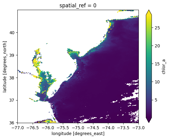
These results can now be easilly stacked

chla = xr.combine_nested(client.gather(futures), concat_dim="time")
chla["time"] = attrs["time"]
chla

<xarray.DataArray 'chlor_a' (time: 16, latitude: 296, longitude: 237)> Size: 4MB
array([[[          nan,           nan,           nan, ...,
                   nan,           nan, 1.0616910e+02],
        [          nan,           nan,           nan, ...,
                   nan,           nan,           nan],
        [          nan,           nan,           nan, ...,
                   nan,           nan,           nan],
        ...,
        [          nan,           nan,           nan, ...,
                   nan,           nan, 6.8380810e-02],
        [          nan,           nan,           nan, ...,
                   nan,           nan, 6.6567786e-02],
        [          nan,           nan,           nan, ...,
                   nan,           nan, 6.5402456e-02]],

       [[          nan,           nan,           nan, ...,
                   nan,           nan,           nan],
        [          nan,           nan,           nan, ...,
                   nan,           nan,           nan],
        [          nan,           nan,           nan, ...,
                   nan,           nan,           nan],
...
                   nan,           nan,           nan],
        [          nan,           nan,           nan, ...,
                   nan,           nan,           nan],
        [          nan,           nan,           nan, ...,
                   nan,           nan,           nan]],

       [[          nan,           nan,           nan, ...,
                   nan,           nan,           nan],
        [          nan,           nan,           nan, ...,
                   nan,           nan,           nan],
        [          nan,           nan,           nan, ...,
                   nan,           nan,           nan],
        ...,
        [          nan,           nan,           nan, ...,
                   nan,           nan,           nan],
        [          nan,           nan,           nan, ...,
                   nan,           nan,           nan],
        [          nan,           nan,           nan, ...,
                   nan,           nan,           nan]]],
      shape=(16, 296, 237), dtype=float32)
Coordinates:
  * longitude    (longitude) float64 2kB -76.99 -76.98 -76.96 ... -73.02 -73.01
  * latitude     (latitude) float64 2kB 40.99 40.97 40.96 ... 36.04 36.02 36.01
    spatial_ref  int64 8B 0
  * time         (time) datetime64[ns] 128B 2024-08-01T17:42:45.090000 ... 20...

xarray.DataArray

'chlor_a'

• time: 16
• latitude: 296
• longitude: 237

• nan nan nan nan nan nan nan nan ... nan nan nan nan nan nan nan nan

  array([[[          nan,           nan,           nan, ...,
                     nan,           nan, 1.0616910e+02],
          [          nan,           nan,           nan, ...,
                     nan,           nan,           nan],
          [          nan,           nan,           nan, ...,
                     nan,           nan,           nan],
          ...,
          [          nan,           nan,           nan, ...,
                     nan,           nan, 6.8380810e-02],
          [          nan,           nan,           nan, ...,
                     nan,           nan, 6.6567786e-02],
          [          nan,           nan,           nan, ...,
                     nan,           nan, 6.5402456e-02]],
  
         [[          nan,           nan,           nan, ...,
                     nan,           nan,           nan],
          [          nan,           nan,           nan, ...,
                     nan,           nan,           nan],
          [          nan,           nan,           nan, ...,
                     nan,           nan,           nan],
  ...
                     nan,           nan,           nan],
          [          nan,           nan,           nan, ...,
                     nan,           nan,           nan],
          [          nan,           nan,           nan, ...,
                     nan,           nan,           nan]],
  
         [[          nan,           nan,           nan, ...,
                     nan,           nan,           nan],
          [          nan,           nan,           nan, ...,
                     nan,           nan,           nan],
          [          nan,           nan,           nan, ...,
                     nan,           nan,           nan],
          ...,
          [          nan,           nan,           nan, ...,
                     nan,           nan,           nan],
          [          nan,           nan,           nan, ...,
                     nan,           nan,           nan],
          [          nan,           nan,           nan, ...,
                     nan,           nan,           nan]]],
        shape=(16, 296, 237), dtype=float32)

• Coordinates: (4)
  • longitude
    (longitude)
    float64
    -76.99 -76.98 ... -73.02 -73.01

    axis :

    X

    long_name :

    longitude

    standard_name :

    longitude

    units :

    degrees_east

    array([-76.992763, -76.975869, -76.958975, ..., -73.039583, -73.02269 ,
           -73.005796], shape=(237,))

  • latitude
    (latitude)
    float64
    40.99 40.97 40.96 ... 36.02 36.01

    axis :

    Y

    long_name :

    latitude

    standard_name :

    latitude

    units :

    degrees_north

    array([40.990906, 40.974012, 40.957118, ..., 36.040984, 36.02409 , 36.007197],
          shape=(296,))

  • spatial_ref
    ()
    int64
    0

    crs_wkt :

    GEOGCS["WGS 84",DATUM["WGS_1984",SPHEROID["WGS 84",6378137,298.257223563,AUTHORITY["EPSG","7030"]],AUTHORITY["EPSG","6326"]],PRIMEM["Greenwich",0,AUTHORITY["EPSG","8901"]],UNIT["degree",0.0174532925199433,AUTHORITY["EPSG","9122"]],AXIS["Latitude",NORTH],AXIS["Longitude",EAST],AUTHORITY["EPSG","4326"]]

    semi_major_axis :

    6378137.0

    semi_minor_axis :

    6356752.314245179

    inverse_flattening :

    298.257223563

    reference_ellipsoid_name :

    WGS 84

    longitude_of_prime_meridian :

    0.0

    prime_meridian_name :

    Greenwich

    geographic_crs_name :

    WGS 84

    horizontal_datum_name :

    World Geodetic System 1984

    grid_mapping_name :

    latitude_longitude

    spatial_ref :

    GEOGCS["WGS 84",DATUM["WGS_1984",SPHEROID["WGS 84",6378137,298.257223563,AUTHORITY["EPSG","7030"]],AUTHORITY["EPSG","6326"]],PRIMEM["Greenwich",0,AUTHORITY["EPSG","8901"]],UNIT["degree",0.0174532925199433,AUTHORITY["EPSG","9122"]],AXIS["Latitude",NORTH],AXIS["Longitude",EAST],AUTHORITY["EPSG","4326"]]

    GeoTransform :

    -77.0012103201517 0.016893931295469684 0.0 40.99935320863791 0.0 -0.016893931295469684

    array(0)

  • time
    (time)
    datetime64[ns]
    2024-08-01T17:42:45.090000 ... 2...

    array(['2024-08-01T17:42:45.090000000', '2024-08-02T16:39:00.164000000',
           '2024-08-02T16:44:00.222000000', '2024-08-02T18:17:18.145000000',
           '2024-08-03T17:13:33.220000000', '2024-08-03T17:18:33.103000000',
           '2024-08-04T16:14:47.125000000', '2024-08-04T17:48:05.224000000',
           '2024-08-05T16:44:20.124000000', '2024-08-05T16:49:20.182000000',
           '2024-08-05T18:22:39.158000000', '2024-08-06T17:18:53.181000000',
           '2024-08-06T17:23:53.063000000', '2024-08-07T16:20:07.086000000',
           '2024-08-07T17:53:25.185000000', '2024-08-07T17:58:25.067000000'],
          dtype='datetime64[ns]')

• Indexes: (3)
  • longitude
    PandasIndex

    PandasIndex(Index([-76.99276335450396,  -76.9758694232085, -76.95897549191302,
           -76.94208156061755, -76.92518762932208, -76.90829369802661,
           -76.89139976673114, -76.87450583543567,  -76.8576119041402,
           -76.84071797284474,
           ...
           -73.15784095043234, -73.14094701913687,  -73.1240530878414,
           -73.10715915654593, -73.09026522525046, -73.07337129395499,
           -73.05647736265952, -73.03958343136406,  -73.0226895000686,
           -73.00579556877312],
          dtype='float64', name='longitude', length=237))

  • latitude
    PandasIndex

    PandasIndex(Index([ 40.99090624299018,  40.97401231169471,  40.95711838039924,
           40.940224449103766, 40.923330517808296,  40.90643658651283,
            40.88954265521736,  40.87264872392189,  40.85575479262642,
            40.83886086133095,
           ...
            36.15924189248585,  36.14234796119038,  36.12545402989491,
            36.10856009859944,  36.09166616730397,   36.0747722360085,
            36.05787830471303,  36.04098437341756,  36.02409044212209,
           36.007196510826624],
          dtype='float64', name='latitude', length=296))

  • time
    PandasIndex

    PandasIndex(DatetimeIndex(['2024-08-01 17:42:45.090000', '2024-08-02 16:39:00.164000',
                   '2024-08-02 16:44:00.222000', '2024-08-02 18:17:18.145000',
                   '2024-08-03 17:13:33.220000', '2024-08-03 17:18:33.103000',
                   '2024-08-04 16:14:47.125000', '2024-08-04 17:48:05.224000',
                   '2024-08-05 16:44:20.124000', '2024-08-05 16:49:20.182000',
                   '2024-08-05 18:22:39.158000', '2024-08-06 17:18:53.181000',
                   '2024-08-06 17:23:53.063000', '2024-08-07 16:20:07.086000',
                   '2024-08-07 17:53:25.185000', '2024-08-07 17:58:25.067000'],
                  dtype='datetime64[ns]', name='time', freq=None))

• Attributes: (0)

plot = chla.mean("time").plot.imshow(robust=True)

client.close()

back to top

5. Scaling Out

The example above relies on a LocalCluster, which only uses the resources on the JupyterLab server running your notebook. The promise of the commercial cloud is massive scalability. Again, dask and the CryoCloud come to our aid in the form of a pre-configured dask_gateway.Gateway. The gateway object created below works with the CryoCloud to launch additional servers, and now those servers are enlisted in your cluster.

from dask_gateway import Gateway

gateway = Gateway()
options = gateway.cluster_options()
options

cluster = gateway.new_cluster(options)
cluster

The cluster starts with no workers, and you must set manual or adaptive scaling in order to get any workers.

The cluster can take several minutes to spin up. Monitor the dashboard to ensure you have workers.

client = cluster.get_client()
client

Client

Client-97f811f9-7221-11f0-8863-86640707dd06

Connection method: Cluster object	Cluster type: dask_gateway.GatewayCluster
Dashboard: /services/dask-gateway/clusters/prod.899a01c54ac14b97acc2bbc1f5b6d35b/status

Launch dashboard in JupyterLab

Cluster Info

GatewayCluster

• Name: prod.899a01c54ac14b97acc2bbc1f5b6d35b
• Dashboard: /services/dask-gateway/clusters/prod.899a01c54ac14b97acc2bbc1f5b6d35b/status

Use this client exactly as above:

futures = client.map(
    grid_match,
    paths,
    dst_crs=crs,
    dst_shape=shape,
    dst_transform=transform,
)

chla = xr.combine_nested(client.gather(futures), concat_dim="time")
chla["time"] = attrs["time"]
chla

cluster.close()

back to top