Orientation to Earthdata Cloud Access#
Tutorial Lead: Anna Windle (NASA, SSAI)
An Earthdata Login account is required to access data from the NASA Earthdata system, including NASA ocean color data.
Summary#
In this example we will use the earthaccess package to search for
OCI products on NASA Earthdata. The earthaccess package, published
on the Python Package Index and conda-forge,
facilitates discovery and use of all NASA Earth Science data
products by providing an abstraction layer for NASA’s Common
Metadata Repository (CMR) API and by simplifying requests to
NASA’s Earthdata Cloud. Searching for data is more
approachable using earthaccess than low-level HTTP requests, and
the same goes for S3 requests.
In short, earthaccess helps authenticate with an Earthdata Login,
makes search easier, and provides a stream-lined way to load
data into xarray containers. For more on earthaccess, visit
the documentation site. Be aware that
earthaccess is under active development.
To understand the discussions below on downloading and opening data, we need to clearly understand where our notebook is running. There are three cases to distinguish:
The notebook is running on the local host. For instance, you started a Jupyter server on your laptop.
The notebook is running on a remote host, but it does not have direct access to the AWS us-west-2 region. For instance, you are running in GitHub Codespaces, which is run on Microsoft Azure.
The notebook is running on a remote host that does have direct access to the NASA Earthdata Cloud (AWS us-west-2 region). This is the case for the PACE Hackweek.
Learning Objectives#
At the end of this notebook you will know:
How to store your NASA Earthdata Login credentials with
earthaccessHow to use
earthaccessto search for OCI data using search filtersHow to download OCI data, but only when you need to
Contents#
1. Setup#
We begin by importing the packages used in this notebook.
import earthaccess
import xarray as xr
from xarray.backends.api import open_datatree
import matplotlib.pyplot as plt
import cartopy.crs as ccrs
import numpy as np
The last import provides a preview of the DataTree object. Once it is fully integrated into XArray,
the additional import won’t be needed, as the function will be available as xr.open_datree.
2. NASA Earthdata Authentication#
Next, we authenticate using our Earthdata Login
credentials. Authentication is not needed to search publicaly
available collections in Earthdata, but is always needed to access
data. We can use the login method from the earthaccess
package. This will create an authenticated session when we provide a
valid Earthdata Login username and password. The earthaccess
package will search for credentials defined by environmental
variables or within a .netrc file saved in the home
directory. If credentials are not found, an interactive prompt will
allow you to input credentials.
The persist=True argument ensures any discovered credentials are
stored in a .netrc file, so the argument is not necessary (but
it’s also harmless) for subsequent calls to earthaccess.login.
auth = earthaccess.login(persist=True)
3. Search for Data#
Collections on NASA Earthdata are discovered with the
search_datasets function, which accepts an instrument filter as an
easy way to get started. Each of the items in the list of
collections returned has a “short-name”.
results = earthaccess.search_datasets(instrument="oci")
for item in results:
    summary = item.summary()
    print(summary["short-name"])
PACE_OCI_L0_SCI
PACE_OCI_L1A_SCI
PACE_OCI_L1B_SCI
PACE_OCI_L1C_SCI
PACE_OCI_L2_AOP_NRT
PACE_OCI_L2_BGC_NRT
PACE_OCI_L2_IOP_NRT
PACE_OCI_L2_PAR_NRT
PACE_OCI_L3B_CHL_NRT
PACE_OCI_L3B_IOP_NRT
PACE_OCI_L3B_KD_NRT
PACE_OCI_L3B_PAR_NRT
PACE_OCI_L3B_POC_NRT
PACE_OCI_L3B_RRS_NRT
PACE_OCI_L3M_CHL_NRT
PACE_OCI_L3M_IOP_NRT
PACE_OCI_L3M_KD_NRT
PACE_OCI_L3M_PAR_NRT
PACE_OCI_L3M_POC_NRT
PACE_OCI_L3M_RRS_NRT
Next, we use the search_data function to find granules within a
collection. Let’s use the short_name for the PACE/OCI Level-2 near real time (NRT), product for biogeochemical properties (although you can
search for granules accross collections too).
The count argument limits the number of granules whose metadata is returned and stored in the results list.
results = earthaccess.search_data(
    short_name="PACE_OCI_L2_BGC_NRT",
    count=1,
)
We can refine our search by passing more parameters that describe
the spatiotemporal domain of our use case. Here, we use the
temporal parameter to request a date range and the bounding_box
parameter to request granules that intersect with a bounding box. We
can even provide a cloud_cover threshold to limit files that have
a lower percetnage of cloud cover. We do not provide a count, so
we’ll get all granules that satisfy the constraints.
tspan = ("2024-07-01", "2024-07-31")
bbox = (-76.75, 36.97, -75.74, 39.01)
clouds = (0, 50)
results = earthaccess.search_data(
    short_name="PACE_OCI_L2_BGC_NRT",
    temporal=tspan,
    bounding_box=bbox,
    cloud_cover=clouds,
)
Displaying results shows the direct download link: try it! The link will download one granule to your local machine, which may or may not be what you want to do. Even if you are running the notebook on a remote host, this download link will open a new browser tab or window and offer to save a file to your local machine. If you are running the notebook locally, this may be of use. However, in the next section we’ll see how to download all the results with one command.
results[0]

results[1]

results[2]

4. Open L2 Data#
Let’s go ahead and open a couple granules using xarray. The earthaccess.open function is used when you want to directly read bytes from a remote filesystem, but not download a whole file. When
running code on a host with direct access to the NASA Earthdata
Cloud, you don’t need to download the data and earthaccess.open
is the way to go.
paths = earthaccess.open(results)
The paths list contains references to files on a remote filesystem. The ob-cumulus-prod-public is the S3 Bucket in AWS us-west-2 region.
paths
[<File-like object S3FileSystem, ob-cumulus-prod-public/PACE_OCI.20240701T175112.L2.OC_BGC.V2_0.NRT.nc>,
 <File-like object S3FileSystem, ob-cumulus-prod-public/PACE_OCI.20240711T170428.L2.OC_BGC.V2_0.NRT.nc>,
 <File-like object S3FileSystem, ob-cumulus-prod-public/PACE_OCI.20240715T174440.L2.OC_BGC.V2_0.NRT.nc>,
 <File-like object S3FileSystem, ob-cumulus-prod-public/PACE_OCI.20240716T164059.L2.OC_BGC.V2_0.NRT.nc>]
dataset = xr.open_dataset(paths[0])
dataset
<xarray.Dataset> Size: 0B
Dimensions:  ()
Data variables:
    *empty*
Attributes: (12/45)
    title:                             OCI Level-2 Data BGC
    product_name:                      PACE_OCI.20240701T175112.L2.OC_BGC.V2_...
    processing_version:                2.0
    history:                           l2gen par=/data6/sdpsoper/vdc/vpu5/wor...
    instrument:                        OCI
    platform:                          PACE
    ...                                ...
    geospatial_lon_max:                -63.887604
    geospatial_lon_min:                -99.13216
    startDirection:                    Ascending
    endDirection:                      Ascending
    day_night_flag:                    Day
earth_sun_distance_correction: 0.9674437642097473- title :
- OCI Level-2 Data BGC
- product_name :
- PACE_OCI.20240701T175112.L2.OC_BGC.V2_0.NRT.nc
- processing_version :
- 2.0
- history :
- l2gen par=/data6/sdpsoper/vdc/vpu5/workbuf/PACE_OCI.20240701T175112.L1B.V2.nc.param metafile=PACE_OCI.20240701T175112.L2.OC_BGC.V2_0.NRT.nc.meta
- instrument :
- OCI
- platform :
- PACE
- Conventions :
- CF-1.8 ACDD-1.3
- license :
- https://science.nasa.gov/earth-science/earth-science-data/data-information-policy/
- naming_authority :
- gov.nasa.gsfc.sci.oceandata
- id :
- 2.0/L2/PACE_OCI.20240701T175112.L2.OC_BGC.V2_0.NRT.nc
- date_created :
- 2024-07-01T21:04:46.000Z
- standard_name_vocabulary :
- CF Standard Name Table v36
- institution :
- NASA Goddard Space Flight Center, Ocean Ecology Laboratory, Ocean Biology Processing Group
- creator_name :
- NASA/GSFC/OBPG
- creator_email :
- data@oceancolor.gsfc.nasa.gov
- creator_url :
- https://oceandata.sci.gsfc.nasa.gov
- project :
- Ocean Biology Processing Group (NASA/GSFC/OBPG)
- publisher_name :
- NASA/GSFC/OBPG
- publisher_url :
- https://oceandata.sci.gsfc.nasa.gov
- publisher_email :
- data@oceancolor.gsfc.nasa.gov
- identifier_product_doi_authority :
- http://dx.doi.org
- identifier_product_doi :
- 10.5067/PACE/OCI/L2/OC_BGC/2.0
- processing_level :
- L2
- cdm_data_type :
- swath
- spatialResolution :
- 1000 m
- time_coverage_start :
- 2024-07-01T17:51:12.132Z
- time_coverage_end :
- 2024-07-01T17:56:12.015Z
- start_center_longitude :
- -77.498215
- start_center_latitude :
- 28.435236
- end_center_longitude :
- -82.93099
- end_center_latitude :
- 46.5052
- northernmost_latitude :
- 48.76455
- southernmost_latitude :
- 25.622993
- easternmost_longitude :
- -63.887604
- westernmost_longitude :
- -99.13216
- geospatial_lat_units :
- degrees_north
- geospatial_lon_units :
- degrees_east
- geospatial_lat_max :
- 48.76455
- geospatial_lat_min :
- 25.622993
- geospatial_lon_max :
- -63.887604
- geospatial_lon_min :
- -99.13216
- startDirection :
- Ascending
- endDirection :
- Ascending
- day_night_flag :
- Day
- earth_sun_distance_correction :
- 0.9674437642097473
Notice that this xarray.Dataset has nothing but “Attributes”. The NetCDF data model includes multi-group hierarchies within a single file, where each group maps to an xarray.Dataset. The whole file maps to a DataTree, which we will only use lightly because the implementation in XArray remains under development.
datatree = open_datatree(paths[0])
datatree
<xarray.DatasetView> Size: 0B
Dimensions:  ()
Data variables:
    *empty*
Attributes: (12/45)
    title:                             OCI Level-2 Data BGC
    product_name:                      PACE_OCI.20240701T175112.L2.OC_BGC.V2_...
    processing_version:                2.0
    history:                           l2gen par=/data6/sdpsoper/vdc/vpu5/wor...
    instrument:                        OCI
    platform:                          PACE
    ...                                ...
    geospatial_lon_max:                -63.887604
    geospatial_lon_min:                -99.13216
    startDirection:                    Ascending
    endDirection:                      Ascending
    day_night_flag:                    Day
earth_sun_distance_correction: 0.9674437642097473<xarray.DatasetView> Size: 11kB Dimensions: (number_of_bands: 286, number_of_reflective_bands: 286) Dimensions without coordinates: number_of_bands, number_of_reflective_bands Data variables: wavelength (number_of_bands) float64 2kB ... vcal_gain (number_of_reflective_bands) float32 1kB ... vcal_offset (number_of_reflective_bands) float32 1kB ... F0 (number_of_reflective_bands) float32 1kB ... aw (number_of_reflective_bands) float32 1kB ... bbw (number_of_reflective_bands) float32 1kB ... k_oz (number_of_reflective_bands) float32 1kB ... k_no2 (number_of_reflective_bands) float32 1kB ... Tau_r (number_of_reflective_bands) float32 1kB ...sensor_band_parameters- number_of_bands: 286
- number_of_reflective_bands: 286
- wavelength(number_of_bands)float64...
- long_name :
- wavelengths
- units :
- nm
- valid_min :
- 0
- valid_max :
- 20000
[286 values with dtype=float64]
- vcal_gain(number_of_reflective_bands)float32...
- long_name :
- Vicarious Calibration Gain
- valid_min :
- 0.0
- valid_max :
- 2.0
[286 values with dtype=float32]
- vcal_offset(number_of_reflective_bands)float32...
- long_name :
- Vicarious Calibration Offset
- units :
- mW cm^-2 um^-1 sr^-1
- valid_min :
- 0.0
- valid_max :
- 10.0
[286 values with dtype=float32]
- F0(number_of_reflective_bands)float32...
- long_name :
- Mean Solar Flux
- units :
- W m^-2 um^-1
- valid_min :
- 0.0
- valid_max :
- 250.0
[286 values with dtype=float32]
- aw(number_of_reflective_bands)float32...
- long_name :
- Band-pass averaged absorption coefficient for seawater
- units :
- m^-1
- standard_name :
- volume_absorption_coefficient_of_radiative_flux_in_sea_water
- valid_min :
- 1e-04
- valid_max :
- 5.0
- reference :
- Pope, R.M. and Fry, E.S., 1997, "Absorption spectrum (380-700 nm) of pure water. II. Integrating cavity measurements," Appl. Opt.,36, 8710-8723.; Kou, L., Labrie, D., Chylek, P., 1993, "Refractive indices of water and ice in the 0.65-2.5 m spectral range," Appl. Opt.,32, 3531-3540 (1993).
[286 values with dtype=float32]
- bbw(number_of_reflective_bands)float32...
- long_name :
- Band-pass averaged backscattering coefficient for seawater
- units :
- m^-1
- standard_name :
- volume_backwards_scattering_coefficient_of_radiative_flux_in_sea_water
- valid_min :
- 5e-06
- valid_max :
- 1.0
- reference :
- Zhang, X., Hu, L., and He, M.-X. (2009). Scattering by pure seawater: effect of salinity, Opt. Express 17(7)
- comment :
- These are nominal values for a salinity of 38.4 at 20 degrees C. The bbw values used in the processing are corrected for temperature and salinity on a per pixel basis.
[286 values with dtype=float32]
- k_oz(number_of_reflective_bands)float32...
- long_name :
- Ozone Absorption cross-sections
- units :
- cm^-1
- valid_min :
- 0.0
- valid_max :
- 0.1
- reference :
- Anderson, S.M., Morton, J., and Mauersberger, K.. "Near-infrared absorption spectra of 16O3 and 18O3: Adiabatic energy of the 1A2 state?." The Journal of Chemical Physics 93.6 (1990): 3826-3832.; Anderson, Stuart M., Maeder, J., and Mauersberger, K. "Effect of isotopic substitution on the visible absorption spectrum of ozone." The Journal of chemical physics 94.10 (1991): 6351-6357; http://dx.doi.org/10.1029/92GL00780; http://dx.doi.org/10.1029/93GL01765; http://dx.doi.org/10.1029/93GL02311
- comment :
- Computed at 229.15K with code provided by E.P.Shettle, NRL, Washington, DC; Based on the measurements of: S.Anderson et al. and J. Burkholder and Talukdar (1994)
[286 values with dtype=float32]
- k_no2(number_of_reflective_bands)float32...
- long_name :
- NO2 Absorption cross-sections
- units :
- cm^2 molecule^-1
- valid_min :
- 0.0
- valid_max :
- 0.1
- reference :
- K. Bogumil, et al., "Measurements of molecular absorption spectra with the SCIAMACHY pre-flight model: Instrument characterization and reference data for atmospheric remote sensing in the 230-2380 nm region," J. Photochem. Photobiol. A.: Photochem. 157, 167-184 (2003).; W. Schneider,et al., "Absorption cross-sections of NO2 in the UV and visible region (200 - 700 nm) at 298 K", J. Photochem. Photobiol. 40, 195-217 (1987)
[286 values with dtype=float32]
- Tau_r(number_of_reflective_bands)float32...
- long_name :
- Rayleigh Optical Thickness
- valid_min :
- 0.0
- valid_max :
- 0.5
- reference :
- Bodhaine, B.A., Wood, N.B, Dutton, E.G., Slusser, J.R. (1999). On Rayleigh Optical Depth Calculations, J. Atmos. Ocean Tech., 16, 1854-1861.
[286 values with dtype=float32]
<xarray.DatasetView> Size: 103kB Dimensions: (number_of_lines: 1710) Dimensions without coordinates: number_of_lines Data variables: year (number_of_lines) float64 14kB ... day (number_of_lines) timedelta64[ns] 14kB ... msec (number_of_lines) timedelta64[ns] 14kB ... detnum (number_of_lines) float32 7kB ... mside (number_of_lines) float32 7kB ... slon (number_of_lines) float32 7kB ... clon (number_of_lines) float32 7kB ... elon (number_of_lines) float32 7kB ... slat (number_of_lines) float32 7kB ... clat (number_of_lines) float32 7kB ... elat (number_of_lines) float32 7kB ... csol_z (number_of_lines) float32 7kB ...scan_line_attributes- number_of_lines: 1710
- year(number_of_lines)float64...
- long_name :
- Scan year
- units :
- years
- valid_min :
- 1900
- valid_max :
- 2100
[1710 values with dtype=float64]
- day(number_of_lines)timedelta64[ns]...
- long_name :
- Scan day of year
- valid_min :
- 0
- valid_max :
- 366
[1710 values with dtype=timedelta64[ns]]
- msec(number_of_lines)timedelta64[ns]...
- long_name :
- Scan time, milliseconds of day
- valid_min :
- 0
- valid_max :
- 86400000
[1710 values with dtype=timedelta64[ns]]
- detnum(number_of_lines)float32...
- long_name :
- Detector Number (zero-based)
- valid_min :
- 0
- valid_max :
- 25
[1710 values with dtype=float32]
- mside(number_of_lines)float32...
- long_name :
- Mirror Side (zero-based)
- valid_min :
- 0
- valid_max :
- 1
[1710 values with dtype=float32]
- slon(number_of_lines)float32...
- long_name :
- Starting Longitude
- units :
- degrees_east
- standard_name :
- longitude
- valid_min :
- -180.0
- valid_max :
- 180.0
[1710 values with dtype=float32]
- clon(number_of_lines)float32...
- long_name :
- Center Longitude
- units :
- degrees_east
- standard_name :
- longitude
- valid_min :
- -180.0
- valid_max :
- 180.0
[1710 values with dtype=float32]
- elon(number_of_lines)float32...
- long_name :
- Ending Longitude
- units :
- degrees_east
- standard_name :
- longitude
- valid_min :
- -180.0
- valid_max :
- 180.0
[1710 values with dtype=float32]
- slat(number_of_lines)float32...
- long_name :
- Starting Latitude
- units :
- degrees_north
- standard_name :
- latitude
- valid_min :
- -90.0
- valid_max :
- 90.0
[1710 values with dtype=float32]
- clat(number_of_lines)float32...
- long_name :
- Center Latitude
- units :
- degrees_north
- standard_name :
- latitude
- valid_min :
- -90.0
- valid_max :
- 90.0
[1710 values with dtype=float32]
- elat(number_of_lines)float32...
- long_name :
- Ending Latitude
- units :
- degrees_north
- standard_name :
- latitude
- valid_min :
- -90.0
- valid_max :
- 90.0
[1710 values with dtype=float32]
- csol_z(number_of_lines)float32...
- long_name :
- Center Solar Zenith Angle
- units :
- degree
- valid_min :
- -90.0
- valid_max :
- 90.0
[1710 values with dtype=float32]
<xarray.DatasetView> Size: 52MB Dimensions: (number_of_lines: 1710, pixels_per_line: 1272) Dimensions without coordinates: number_of_lines, pixels_per_line Data variables: chlor_a (number_of_lines, pixels_per_line) float32 9MB ... carbon_phyto (number_of_lines, pixels_per_line) float32 9MB ... poc (number_of_lines, pixels_per_line) float32 9MB ... chlor_a_unc (number_of_lines, pixels_per_line) float32 9MB ... carbon_phyto_unc (number_of_lines, pixels_per_line) float32 9MB ... l2_flags (number_of_lines, pixels_per_line) int32 9MB ...geophysical_data- number_of_lines: 1710
- pixels_per_line: 1272
- chlor_a(number_of_lines, pixels_per_line)float32...
- long_name :
- Chlorophyll Concentration, OCI Algorithm
- units :
- mg m^-3
- standard_name :
- mass_concentration_of_chlorophyll_in_sea_water
- valid_min :
- 0.001
- valid_max :
- 100.0
- reference :
- Hu, C., Lee Z., and Franz, B.A. (2012). Chlorophyll-a algorithms for oligotrophic oceans: A novel approach based on three-band reflectance difference, J. Geophys. Res., 117, C01011, doi:10.1029/2011JC007395.
[2175120 values with dtype=float32]
- carbon_phyto(number_of_lines, pixels_per_line)float32...
- long_name :
- Phytoplankton Carbon
- units :
- mg m^-3
- valid_min :
- 0.0
- valid_max :
- 1000.0
- reference :
- Graff, J.R., Westberry, T.K., Milligan, A.J., Brown, M.B., Dall'Olmo, G., Dongen-Vogels, V.v., Reifel, K.M., and Behrenfeld, M.J. (2015). Analytical phytoplankton carbon measurements spanning diverse ecosystems. Deep Sea Research Part I: Oceanographic Research Papers, 102, 16-25
[2175120 values with dtype=float32]
- poc(number_of_lines, pixels_per_line)float32...
- long_name :
- Particulate Organic Carbon, D. Stramski, 2022 (hybrid version)
- units :
- mg m^-3
- valid_min :
- -32000
- valid_max :
- -22000
- reference :
- Stramski, D., et al. "Ocean color algorithms to estimate the concentration of particulate organic carbon in surface waters of the global ocean in support of a long-term data record from multiple satellite missions." Remote Sensing of Environment 269 (2022)
[2175120 values with dtype=float32]
- chlor_a_unc(number_of_lines, pixels_per_line)float32...
- long_name :
- Uncertainty in chlorophyll a concentration
- units :
- mg m^-3
- standard_name :
- chlorophyll_concentration_in_sea_water standard_error
- valid_min :
- 0.001
- valid_max :
- 100.0
[2175120 values with dtype=float32]
- carbon_phyto_unc(number_of_lines, pixels_per_line)float32...
- long_name :
- Phytoplankton Carbon standard uncertainty
- units :
- mg m^-3
- valid_min :
- 0.0
- valid_max :
- 1000.0
- reference :
- Graff, J.R., Westberry, T.K., Milligan, A.J., Brown, M.B., Dall'Olmo, G., Dongen-Vogels, V.v., Reifel, K.M., and Behrenfeld, M.J. (2015). Analytical phytoplankton carbon measurements spanning diverse ecosystems. Deep Sea Research Part I: Oceanographic Research Papers, 102, 16-25
[2175120 values with dtype=float32]
- l2_flags(number_of_lines, pixels_per_line)int32...
- long_name :
- Level-2 Processing Flags
- valid_min :
- -2147483648
- valid_max :
- 2147483647
- flag_masks :
- [ 1 2 4 8 16 32 64 128 256 512 1024 2048 4096 8192 16384 32768 65536 131072 262144 524288 1048576 2097152 4194304 8388608 16777216 33554432 67108864 134217728 268435456 536870912 1073741824 -2147483648]
- flag_meanings :
- ATMFAIL LAND PRODWARN HIGLINT HILT HISATZEN COASTZ SPARE STRAYLIGHT CLDICE COCCOLITH TURBIDW HISOLZEN SPARE LOWLW CHLFAIL NAVWARN ABSAER SPARE MAXAERITER MODGLINT CHLWARN ATMWARN SPARE SEAICE NAVFAIL FILTER SPARE BOWTIEDEL HIPOL PRODFAIL SPARE
[2175120 values with dtype=int32]
<xarray.DatasetView> Size: 17MB Dimensions: (number_of_lines: 1710, pixels_per_line: 1272) Dimensions without coordinates: number_of_lines, pixels_per_line Data variables: longitude (number_of_lines, pixels_per_line) float32 9MB ... latitude (number_of_lines, pixels_per_line) float32 9MB ... tilt (number_of_lines) float32 7kB ... Attributes: gringpointlongitude: [-90.67664 -63.887604 -65.21011 -99.13216 ] gringpointlatitude: [25.622993 30.946634 48.76455 42.731358] gringpointsequence: [1 2 3 4]navigation_data- number_of_lines: 1710
- pixels_per_line: 1272
- longitude(number_of_lines, pixels_per_line)float32...
- long_name :
- Longitude
- units :
- degrees_east
- standard_name :
- longitude
- valid_min :
- -180.0
- valid_max :
- 180.0
[2175120 values with dtype=float32]
- latitude(number_of_lines, pixels_per_line)float32...
- long_name :
- Latitude
- units :
- degrees_north
- standard_name :
- latitude
- valid_min :
- -90.0
- valid_max :
- 90.0
[2175120 values with dtype=float32]
- tilt(number_of_lines)float32...
- long_name :
- Sensor tilt angle
- units :
- degree
- valid_min :
- -25.0
- valid_max :
- 25.0
[1710 values with dtype=float32]
- gringpointlongitude :
- [-90.67664 -63.887604 -65.21011 -99.13216 ]
- gringpointlatitude :
- [25.622993 30.946634 48.76455 42.731358]
- gringpointsequence :
- [1 2 3 4]
<xarray.DatasetView> Size: 0B Dimensions: () Data variables: *empty* Attributes: software_name: l2gen software_version: 9.7.0-V2024.0 input_sources: PACE_OCI.20240701T175112.L1B.V2.nc,GMAO_IT.20240701T14... calibration_data: mask_names: ATMFAIL,LAND,CLDICE,HILTprocessing_control<xarray.DatasetView> Size: 0B Dimensions: () Data variables: *empty* Attributes: (12/248) ifile: PACE_OCI.20240701T175112.L1B.V2.nc ofile: PACE_OCI.20240701T175112.L2.OC_BGC.V2_0.NRT.nc l2prod: chlor_a carbon_phyto poc chlor_a_unc carbon_phyto_unc oformat: netCDF4 oformat_depth: 8bit fqfile: $OCDATAROOT/common/morel_fq.nc ... ... spixl: 1 epixl: -1 dpixl: 1 sline: 1 eline: -1 dline: 1input_parameters- ifile :
- PACE_OCI.20240701T175112.L1B.V2.nc
- ofile :
- PACE_OCI.20240701T175112.L2.OC_BGC.V2_0.NRT.nc
- l2prod :
- chlor_a carbon_phyto poc chlor_a_unc carbon_phyto_unc
- oformat :
- netCDF4
- oformat_depth :
- 8bit
- fqfile :
- $OCDATAROOT/common/morel_fq.nc
- parfile :
- geofile :
- gmpfile :
- metafile :
- PACE_OCI.20240701T175112.L2.OC_BGC.V2_0.NRT.nc.meta
- suite :
- BGC
- mode :
- 0
- deflate :
- 4
- proc_ocean :
- 1
- proc_land :
- 1
- proc_cloud :
- 0
- proc_uncertainty :
- 1
- proc_sst :
- 0
- atmocor :
- 1
- seawater_opt :
- 1
- aermodfile :
- $OCDATAROOT/oci/aerosol/aerosol_oci
- uncertaintyfile :
- $OCDATAROOT/oci/uncertainty.nc
- aer_opt :
- -18
- aer_wave_short :
- 751
- aer_wave_long :
- 870
- aer_wave_base :
- 870
- aer_swir_short :
- -1
- aer_swir_long :
- -1
- aer_rrs_short :
- -1.00000
- aer_rrs_long :
- -1.00000
- aer_angstrom :
- -999.00000
- aer_iter_max :
- 10
- brdf_opt :
- 7
- gas_opt :
- 491
- atrem_opt :
- 0
- atrem_full :
- 0
- atrem_geom :
- 0
- atrem_model :
- 0
- atrem_splitpaths :
- 0
- iop_opt :
- 0
- cphyt_opt :
- 1
- gsm_opt :
- 0
- gsm_fit :
- 0
- gsm_adg_s :
- 0.02061
- gsm_bbp_s :
- 1.03373
- gsm_aphw :
- 412.00000, 443.00000, 490.00000, 510.00000, 555.00000, 670.00000, -1.00000, -1.00000, -1.00000, -1.00000, -1.00000, -1.00000, -1.00000, -1.00000, -1.00000, -1.00000, -1.00000, -1.00000, -1.00000, -1.00000, -1.00000, -1.00000, -1.00000, -1.00000, -1.00000, -1.00000, -1.00000, -1.00000, -1.00000, -1.00000, -1.00000, -1.00000, -1.00000, -1.00000, -1.00000, -1.00000, -1.00000, -1.00000, -1.00000, -1.00000, -1.00000, -1.00000, -1.00000, -1.00000, -1.00000, -1.00000, -1.00000, -1.00000, -1.00000, -1.00000, -1.00000, -1.00000, -1.00000, -1.00000, -1.00000, -1.00000, -1.00000, -1.00000, -1.00000, -1.00000, -1.00000, -1.00000, -1.00000, -1.00000, -1.00000, -1.00000, -1.00000, -1.00000, -1.00000, -1.00000, -1.00000, -1.00000, -1.00000, -1.00000, -1.00000, -1.00000, -1.00000, -1.00000, -1.00000, -1.00000, -1.00000, -1.00000, -1.00000, -1.00000, -1.00000, -1.00000, -1.00000, -1.00000, -1.00000, -1.00000, -1.00000, -1.00000, -1.00000, -1.00000, -1.00000, -1.00000, -1.00000, -1.00000, -1.00000, -1.00000, -1.00000, -1.00000, -1.00000, -1.00000, -1.00000, -1.00000, -1.00000, -1.00000, -1.00000, -1.00000, -1.00000, -1.00000, -1.00000, -1.00000, -1.00000, -1.00000, -1.00000, -1.00000, -1.00000, -1.00000, -1.00000, -1.00000, -1.00000, -1.00000, -1.00000, -1.00000, -1.00000, -1.00000, -1.00000, -1.00000, -1.00000, -1.00000, -1.00000, -1.00000, -1.00000, -1.00000, -1.00000, -1.00000, -1.00000, -1.00000, -1.00000, -1.00000, -1.00000, -1.00000, -1.00000, -1.00000, -1.00000, -1.00000, -1.00000, -1.00000, -1.00000, -1.00000, -1.00000, -1.00000, -1.00000, -1.00000, -1.00000, -1.00000, -1.00000, -1.00000, -1.00000, -1.00000, -1.00000, -1.00000, -1.00000, -1.00000, -1.00000, -1.00000, -1.00000, -1.00000, -1.00000, -1.00000, -1.00000, -1.00000, -1.00000, -1.00000, -1.00000, -1.00000, -1.00000, -1.00000, -1.00000, -1.00000, -1.00000, -1.00000, -1.00000, -1.00000, -1.00000, -1.00000, -1.00000, -1.00000, -1.00000, -1.00000, -1.00000, -1.00000, -1.00000, -1.00000, -1.00000, -1.00000, -1.00000, -1.00000, -1.00000, -1.00000, -1.00000, -1.00000, -1.00000, -1.00000, -1.00000, -1.00000, -1.00000, -1.00000, -1.00000, -1.00000, -1.00000, -1.00000, -1.00000, -1.00000, -1.00000, -1.00000, -1.00000, -1.00000, -1.00000, -1.00000, -1.00000, -1.00000, -1.00000, -1.00000, -1.00000, -1.00000, -1.00000, -1.00000, -1.00000, -1.00000, -1.00000, -1.00000, -1.00000, -1.00000, -1.00000, -1.00000, -1.00000, -1.00000, -1.00000, -1.00000, -1.00000, -1.00000, -1.00000, -1.00000, -1.00000, -1.00000, -1.00000, -1.00000, -1.00000, -1.00000, -1.00000, -1.00000, -1.00000, -1.00000, -1.00000, -1.00000, -1.00000, -1.00000, -1.00000, -1.00000, -1.00000, -1.00000, -1.00000, -1.00000, -1.00000, -1.00000, -1.00000, -1.00000, -1.00000, -1.00000, -1.00000, -1.00000, -1.00000, -1.00000, -1.00000, -1.00000, -1.00000, -1.00000, -1.00000, -1.00000, -1.00000, -1.00000, -1.00000, -1.00000
- gsm_aphs :
- 0.00665, 0.05582, 0.02055, 0.01910, 0.01015, 0.01424, -1.00000, -1.00000, -1.00000, -1.00000, -1.00000, -1.00000, -1.00000, -1.00000, -1.00000, -1.00000, -1.00000, -1.00000, -1.00000, -1.00000, -1.00000, -1.00000, -1.00000, -1.00000, -1.00000, -1.00000, -1.00000, -1.00000, -1.00000, -1.00000, -1.00000, -1.00000, -1.00000, -1.00000, -1.00000, -1.00000, -1.00000, -1.00000, -1.00000, -1.00000, -1.00000, -1.00000, -1.00000, -1.00000, -1.00000, -1.00000, -1.00000, -1.00000, -1.00000, -1.00000, -1.00000, -1.00000, -1.00000, -1.00000, -1.00000, -1.00000, -1.00000, -1.00000, -1.00000, -1.00000, -1.00000, -1.00000, -1.00000, -1.00000, -1.00000, -1.00000, -1.00000, -1.00000, -1.00000, -1.00000, -1.00000, -1.00000, -1.00000, -1.00000, -1.00000, -1.00000, -1.00000, -1.00000, -1.00000, -1.00000, -1.00000, -1.00000, -1.00000, -1.00000, -1.00000, -1.00000, -1.00000, -1.00000, -1.00000, -1.00000, -1.00000, -1.00000, -1.00000, -1.00000, -1.00000, -1.00000, -1.00000, -1.00000, -1.00000, -1.00000, -1.00000, -1.00000, -1.00000, -1.00000, -1.00000, -1.00000, -1.00000, -1.00000, -1.00000, -1.00000, -1.00000, -1.00000, -1.00000, -1.00000, -1.00000, -1.00000, -1.00000, -1.00000, -1.00000, -1.00000, -1.00000, -1.00000, -1.00000, -1.00000, -1.00000, -1.00000, -1.00000, -1.00000, -1.00000, -1.00000, -1.00000, -1.00000, -1.00000, -1.00000, -1.00000, -1.00000, -1.00000, -1.00000, -1.00000, -1.00000, -1.00000, -1.00000, -1.00000, -1.00000, -1.00000, -1.00000, -1.00000, -1.00000, -1.00000, -1.00000, -1.00000, -1.00000, -1.00000, -1.00000, -1.00000, -1.00000, -1.00000, -1.00000, -1.00000, -1.00000, -1.00000, -1.00000, -1.00000, -1.00000, -1.00000, -1.00000, -1.00000, -1.00000, -1.00000, -1.00000, -1.00000, -1.00000, -1.00000, -1.00000, -1.00000, -1.00000, -1.00000, -1.00000, -1.00000, -1.00000, -1.00000, -1.00000, -1.00000, -1.00000, -1.00000, -1.00000, -1.00000, -1.00000, -1.00000, -1.00000, -1.00000, -1.00000, -1.00000, -1.00000, -1.00000, -1.00000, -1.00000, -1.00000, -1.00000, -1.00000, -1.00000, -1.00000, -1.00000, -1.00000, -1.00000, -1.00000, -1.00000, -1.00000, -1.00000, -1.00000, -1.00000, -1.00000, -1.00000, -1.00000, -1.00000, -1.00000, -1.00000, -1.00000, -1.00000, -1.00000, -1.00000, -1.00000, -1.00000, -1.00000, -1.00000, -1.00000, -1.00000, -1.00000, -1.00000, -1.00000, -1.00000, -1.00000, -1.00000, -1.00000, -1.00000, -1.00000, -1.00000, -1.00000, -1.00000, -1.00000, -1.00000, -1.00000, -1.00000, -1.00000, -1.00000, -1.00000, -1.00000, -1.00000, -1.00000, -1.00000, -1.00000, -1.00000, -1.00000, -1.00000, -1.00000, -1.00000, -1.00000, -1.00000, -1.00000, -1.00000, -1.00000, -1.00000, -1.00000, -1.00000, -1.00000, -1.00000, -1.00000, -1.00000, -1.00000, -1.00000, -1.00000, -1.00000, -1.00000, -1.00000, -1.00000, -1.00000, -1.00000, -1.00000, -1.00000, -1.00000, -1.00000, -1.00000, -1.00000, -1.00000, -1.00000, -1.00000
- qaa_adg_s :
- 0.01500
- qaa_wave :
- 410, 440, 490, 555, 670
- giop_maxiter :
- 50
- giop_fit_opt :
- 1
- giop_aph_opt :
- 2
- giop_acdom_opt :
- 1
- giop_anap_opt :
- 1
- giop_adg_opt :
- 1
- giop_bbp_opt :
- 3
- giop_bbnap_opt :
- 1
- giop_bbph_opt :
- 1
- giop_rrs_opt :
- 0
- giop_rrs_diff :
- 0.33000
- giop_aph_file :
- $OCDATAROOT/common/aph_default.txt
- giop_uaph_file :
- $OCDATAROOT/common/aph_unc_default.txt
- giop_aph_s :
- -1000.00000
- giop_adg_file :
- $OCDATAROOT/common/adg_default.txt
- giop_uadg_file :
- $OCDATAROOT/common/adg_unc_default.txt
- giop_adg_s :
- 0.01800
- giop_uadg_s :
- 0.00000
- giop_bbp_file :
- $OCDATAROOT/common/bbp_default.txt
- giop_bbp_s :
- -1000.00000
- giop_ubbp_s :
- 0.00000
- giop_acdom_file :
- giop_uacdom_file :
- giop_anap_file :
- giop_uanap_file :
- giop_bbph_file :
- giop_ubbph_file :
- giop_bbnap_file :
- giop_ubbnap_file :
- giop_grd :
- 0.09490, 0.07940
- giop_wave :
- 413.0, 442.0, 490.0, 510.0, 555.0, 670.0, -1.0, -1.0, -1.0, -1.0, -1.0, -1.0, -1.0, -1.0, -1.0, -1.0, -1.0, -1.0, -1.0, -1.0, -1.0, -1.0, -1.0, -1.0, -1.0, -1.0, -1.0, -1.0, -1.0, -1.0, -1.0, -1.0, -1.0, -1.0, -1.0, -1.0, -1.0, -1.0, -1.0, -1.0, -1.0, -1.0, -1.0, -1.0, -1.0, -1.0, -1.0, -1.0, -1.0, -1.0, -1.0, -1.0, -1.0, -1.0, -1.0, -1.0, -1.0, -1.0, -1.0, -1.0, -1.0, -1.0, -1.0, -1.0, -1.0, -1.0, -1.0, -1.0, -1.0, -1.0, -1.0, -1.0, -1.0, -1.0, -1.0, -1.0, -1.0, -1.0, -1.0, -1.0, -1.0, -1.0, -1.0, -1.0, -1.0, -1.0, -1.0, -1.0, -1.0, -1.0, -1.0, -1.0, -1.0, -1.0, -1.0, -1.0, -1.0, -1.0, -1.0, -1.0, -1.0, -1.0, -1.0, -1.0, -1.0, -1.0, -1.0, -1.0, -1.0, -1.0, -1.0, -1.0, -1.0, -1.0, -1.0, -1.0, -1.0, -1.0, -1.0, -1.0, -1.0, -1.0, -1.0, -1.0, -1.0, -1.0, -1.0, -1.0, -1.0, -1.0, -1.0, -1.0, -1.0, -1.0, -1.0, -1.0, -1.0, -1.0, -1.0, -1.0, -1.0, -1.0, -1.0, -1.0, -1.0, -1.0, -1.0, -1.0, -1.0, -1.0, -1.0, -1.0, -1.0, -1.0, -1.0, -1.0, -1.0, -1.0, -1.0, -1.0, -1.0, -1.0, -1.0, -1.0, -1.0, -1.0, -1.0, -1.0, -1.0, -1.0, -1.0, -1.0, -1.0, -1.0, -1.0, -1.0, -1.0, -1.0, -1.0, -1.0, -1.0, -1.0, -1.0, -1.0, -1.0, -1.0, -1.0, -1.0, -1.0, -1.0, -1.0, -1.0, -1.0, -1.0, -1.0, -1.0, -1.0, -1.0, -1.0, -1.0, -1.0, -1.0, -1.0, -1.0, -1.0, -1.0, -1.0, -1.0, -1.0, -1.0, -1.0, -1.0, -1.0, -1.0, -1.0, -1.0, -1.0, -1.0, -1.0, -1.0, -1.0, -1.0, -1.0, -1.0, -1.0, -1.0, -1.0, -1.0, -1.0, -1.0, -1.0, -1.0, -1.0, -1.0, -1.0, -1.0, -1.0, -1.0, -1.0, -1.0, -1.0, -1.0, -1.0, -1.0, -1.0, -1.0, -1.0, -1.0, -1.0, -1.0, -1.0, -1.0, -1.0, -1.0, -1.0, -1.0, -1.0, -1.0, -1.0, -1.0, -1.0, -1.0, -1.0, -1.0, -1.0, -1.0, -1.0, -1.0, -1.0, -1.0, -1.0, -1.0, -1.0, -1.0, -1.0, -1.0, -1.0, -1.0, -1.0, -1.0, -1.0, -1.0, -1.0, -1.0, -1.0, -1.0
- giop_rrs_unc_opt :
- 0
- giop_rrs_unc :
- -1.0, -1.0, -1.0, -1.0, -1.0, -1.0, -1.0, -1.0, -1.0, -1.0, -1.0, -1.0, -1.0, -1.0, -1.0, -1.0, -1.0, -1.0, -1.0, -1.0, -1.0, -1.0, -1.0, -1.0, -1.0, -1.0, -1.0, -1.0, -1.0, -1.0, -1.0, -1.0, -1.0, -1.0, -1.0, -1.0, -1.0, -1.0, -1.0, -1.0, -1.0, -1.0, -1.0, -1.0, -1.0, -1.0, -1.0, -1.0, -1.0, -1.0, -1.0, -1.0, -1.0, -1.0, -1.0, -1.0, -1.0, -1.0, -1.0, -1.0, -1.0, -1.0, -1.0, -1.0, -1.0, -1.0, -1.0, -1.0, -1.0, -1.0, -1.0, -1.0, -1.0, -1.0, -1.0, -1.0, -1.0, -1.0, -1.0, -1.0, -1.0, -1.0, -1.0, -1.0, -1.0, -1.0, -1.0, -1.0, -1.0, -1.0, -1.0, -1.0, -1.0, -1.0, -1.0, -1.0, -1.0, -1.0, -1.0, -1.0, -1.0, -1.0, -1.0, -1.0, -1.0, -1.0, -1.0, -1.0, -1.0, -1.0, -1.0, -1.0, -1.0, -1.0, -1.0, -1.0, -1.0, -1.0, -1.0, -1.0, -1.0, -1.0, -1.0, -1.0, -1.0, -1.0, -1.0, -1.0, -1.0, -1.0, -1.0, -1.0, -1.0, -1.0, -1.0, -1.0, -1.0, -1.0, -1.0, -1.0, -1.0, -1.0, -1.0, -1.0, -1.0, -1.0, -1.0, -1.0, -1.0, -1.0, -1.0, -1.0, -1.0, -1.0, -1.0, -1.0, -1.0, -1.0, -1.0, -1.0, -1.0, -1.0, -1.0, -1.0, -1.0, -1.0, -1.0, -1.0, -1.0, -1.0, -1.0, -1.0, -1.0, -1.0, -1.0, -1.0, -1.0, -1.0, -1.0, -1.0, -1.0, -1.0, -1.0, -1.0, -1.0, -1.0, -1.0, -1.0, -1.0, -1.0, -1.0, -1.0, -1.0, -1.0, -1.0, -1.0, -1.0, -1.0, -1.0, -1.0, -1.0, -1.0, -1.0, -1.0, -1.0, -1.0, -1.0, -1.0, -1.0, -1.0, -1.0, -1.0, -1.0, -1.0, -1.0, -1.0, -1.0, -1.0, -1.0, -1.0, -1.0, -1.0, -1.0, -1.0, -1.0, -1.0, -1.0, -1.0, -1.0, -1.0, -1.0, -1.0, -1.0, -1.0, -1.0, -1.0, -1.0, -1.0, -1.0, -1.0, -1.0, -1.0, -1.0, -1.0, -1.0, -1.0, -1.0, -1.0, -1.0, -1.0, -1.0, -1.0, -1.0, -1.0, -1.0, -1.0, -1.0, -1.0, -1.0, -1.0, -1.0, -1.0, -1.0, -1.0, -1.0, -1.0, -1.0, -1.0, -1.0, -1.0, -1.0, -1.0, -1.0, -1.0, -1.0, -1.0, -1.0, -1.0, -1.0, -1.0, -1.0, -1.0, -1.0, -1.0, -1.0, -1.0
- polfile :
- pol_opt :
- 0
- vcnnfile :
- absaer_opt :
- 2
- glint_opt :
- 1
- cirrus_opt :
- 0
- oxaband_opt :
- 2
- filter_opt :
- 1
- filter_file :
- $OCDATAROOT/oci/msl12_filter.dat
- aerfile :
- tgtfile :
- met1 :
- GMAO_IT.20240701T140000.MET.NRT.nc
- met2 :
- GMAO_IT.20240701T140000.MET.NRT.nc
- met3 :
- GMAO_IT.20240701T140000.MET.NRT.nc
- ozone1 :
- GMAO_IT.20240701T140000.MET.NRT.nc
- ozone2 :
- GMAO_IT.20240701T140000.MET.NRT.nc
- ozone3 :
- GMAO_IT.20240701T140000.MET.NRT.nc
- rad1 :
- rad2 :
- rad3 :
- anc_profile1 :
- anc_profile2 :
- anc_profile3 :
- anc_aerosol1 :
- GMAO_IT.20240701T120000.AER.NRT.nc
- anc_aerosol2 :
- GMAO_IT.20240701T120000.AER.NRT.nc
- anc_aerosol3 :
- GMAO_IT.20240701T120000.AER.NRT.nc
- sfc_albedo :
- cth_albedo :
- anc_cor_file :
- $OCDATAROOT/common/anc_cor_file_28jan2014.nc
- pixel_anc_file :
- land :
- $OCDATAROOT/common/gebco_ocssw_v2020.nc
- water :
- $OCDATAROOT/common/gebco_ocssw_v2020.nc
- shallow_water_depth :
- 30.00
- demfile :
- $OCDATAROOT/common/gebco_ocssw_v2020.nc
- dem_auxfile :
- mldfile :
- $OCDATAROOT/common/mld_climatology_woa1994.hdf
- icefile :
- 20240630120000-CMC-L4_GHRSST-SSTfnd-CMC0.1deg-GLOB-v02.0-fv03.0.nc
- sstfile :
- 20240630120000-CMC-L4_GHRSST-SSTfnd-CMC0.1deg-GLOB-v02.0-fv03.0.nc
- sstreftype :
- 0
- sssfile :
- $OCDATAROOT/common/sss_climatology_woa2009.hdf
- no2file :
- $OCDATAROOT/common/no2_climatology_v2013.hdf
- alphafile :
- $OCDATAROOT/common/alpha510_climatology.hdf
- tauafile :
- $OCDATAROOT/common/taua865_climatology.hdf
- picfile :
- $OCDATAROOT/common/calcite_table-20170109.txt
- owmcfile :
- $OCDATAROOT/common/owmc_lut.hdf
- prodxmlfile :
- breflectfile :
- aerbinfile :
- naermodels :
- 80
- aermodels :
- r30f95, r30f80, r30f50, r30f30, r30f20, r30f10, r30f05, r30f02, r30f01, r30f00, r50f95, r50f80, r50f50, r50f30, r50f20, r50f10, r50f05, r50f02, r50f01, r50f00, r70f95, r70f80, r70f50, r70f30, r70f20, r70f10, r70f05, r70f02, r70f01, r70f00, r75f95, r75f80, r75f50, r75f30, r75f20, r75f10, r75f05, r75f02, r75f01, r75f00, r80f95, r80f80, r80f50, r80f30, r80f20, r80f10, r80f05, r80f02, r80f01, r80f00, r85f95, r85f80, r85f50, r85f30, r85f20, r85f10, r85f05, r85f02, r85f01, r85f00, r90f95, r90f80, r90f50, r90f30, r90f20, r90f10, r90f05, r90f02, r90f01, r90f00, r95f95, r95f80, r95f50, r95f30, r95f20, r95f10, r95f05, r95f02, r95f01, r95f00
- taua :
- 0.0000, 0.0000, 0.0000, 0.0000, 0.0000, 0.0000, 0.0000, 0.0000, 0.0000, 0.0000, 0.0000, 0.0000, 0.0000, 0.0000, 0.0000, 0.0000, 0.0000, 0.0000, 0.0000, 0.0000, 0.0000, 0.0000, 0.0000, 0.0000, 0.0000, 0.0000, 0.0000, 0.0000, 0.0000, 0.0000, 0.0000, 0.0000, 0.0000, 0.0000, 0.0000, 0.0000, 0.0000, 0.0000, 0.0000, 0.0000, 0.0000, 0.0000, 0.0000, 0.0000, 0.0000, 0.0000, 0.0000, 0.0000, 0.0000, 0.0000, 0.0000, 0.0000, 0.0000, 0.0000, 0.0000, 0.0000, 0.0000, 0.0000, 0.0000, 0.0000, 0.0000, 0.0000, 0.0000, 0.0000, 0.0000, 0.0000, 0.0000, 0.0000, 0.0000, 0.0000, 0.0000, 0.0000, 0.0000, 0.0000, 0.0000, 0.0000, 0.0000, 0.0000, 0.0000, 0.0000, 0.0000, 0.0000, 0.0000, 0.0000, 0.0000, 0.0000, 0.0000, 0.0000, 0.0000, 0.0000, 0.0000, 0.0000, 0.0000, 0.0000, 0.0000, 0.0000, 0.0000, 0.0000, 0.0000, 0.0000, 0.0000, 0.0000, 0.0000, 0.0000, 0.0000, 0.0000, 0.0000, 0.0000, 0.0000, 0.0000, 0.0000, 0.0000, 0.0000, 0.0000, 0.0000, 0.0000, 0.0000, 0.0000, 0.0000, 0.0000, 0.0000, 0.0000, 0.0000, 0.0000, 0.0000, 0.0000, 0.0000, 0.0000, 0.0000, 0.0000, 0.0000, 0.0000, 0.0000, 0.0000, 0.0000, 0.0000, 0.0000, 0.0000, 0.0000, 0.0000, 0.0000, 0.0000, 0.0000, 0.0000, 0.0000, 0.0000, 0.0000, 0.0000, 0.0000, 0.0000, 0.0000, 0.0000, 0.0000, 0.0000, 0.0000, 0.0000, 0.0000, 0.0000, 0.0000, 0.0000, 0.0000, 0.0000, 0.0000, 0.0000, 0.0000, 0.0000, 0.0000, 0.0000, 0.0000, 0.0000, 0.0000, 0.0000, 0.0000, 0.0000, 0.0000, 0.0000, 0.0000, 0.0000, 0.0000, 0.0000, 0.0000, 0.0000, 0.0000, 0.0000, 0.0000, 0.0000, 0.0000, 0.0000, 0.0000, 0.0000, 0.0000, 0.0000, 0.0000, 0.0000, 0.0000, 0.0000, 0.0000, 0.0000, 0.0000, 0.0000, 0.0000, 0.0000, 0.0000, 0.0000, 0.0000, 0.0000, 0.0000, 0.0000, 0.0000, 0.0000, 0.0000, 0.0000, 0.0000, 0.0000, 0.0000, 0.0000, 0.0000, 0.0000, 0.0000, 0.0000, 0.0000, 0.0000, 0.0000, 0.0000, 0.0000, 0.0000, 0.0000, 0.0000, 0.0000, 0.0000, 0.0000, 0.0000, 0.0000, 0.0000, 0.0000, 0.0000, 0.0000, 0.0000, 0.0000, 0.0000, 0.0000, 0.0000, 0.0000, 0.0000, 0.0000, 0.0000, 0.0000, 0.0000, 0.0000, 0.0000, 0.0000, 0.0000, 0.0000, 0.0000, 0.0000, 0.0000, 0.0000, 0.0000, 0.0000, 0.0000, 0.0000, 0.0000, 0.0000, 0.0000, 0.0000, 0.0000, 0.0000, 0.0000, 0.0000, 0.0000, 0.0000, 0.0000, 0.0000, 0.0000, 0.0000, 0.0000, 0.0000, 0.0000, 0.0000, 0.0000, 0.0000, 0.0000, 0.0000, 0.0000, 0.0000, 0.0000
- aermodrat :
- 0.00000
- aermodmin :
- -1
- aermodmax :
- -1
- cirrus_thresh :
- -1.00000, -1.00000
- absaer :
- 0.000
- rhoamin :
- 0.00020
- nlwmin :
- 0.150
- wsmax :
- 12.000
- coccolith :
- 1.1000, 0.9000, 0.7500, 1.8500, 1.0000, 1.6500, 0.6000, 1.1500
- tauamax :
- 0.300
- epsmin :
- 0.800
- epsmax :
- 1.350
- windspeed :
- -1000.000
- windangle :
- -1000.000
- pressure :
- -1000.000
- ozone :
- -1000.000
- watervapor :
- -1000.000
- relhumid :
- -1000.000
- ice_threshold :
- 0.100
- mumm_alpha :
- 1.945
- mumm_gamma :
- 1.000
- mumm_epsilon :
- 1.000
- chloc2_wave :
- 490, 555
- chloc2_coef :
- 0.25110, -2.08530, 1.50350, -3.17470, 0.33830
- chloc3_wave :
- 442, 490, 555
- chloc3_coef :
- 0.25150, -2.37980, 1.58230, -0.63720, -0.56920
- chloc4_wave :
- 442, 490, 510, 555
- chloc4_coef :
- 0.32814, -3.20725, 3.22969, -1.36769, -0.81739
- avw_coef :
- 0.00000E+00, 0.00000E+00, 0.00000E+00, 0.00000E+00, 0.00000E+00, 0.00000E+00
- kd2_wave :
- 490, 555
- kd2_coef :
- 0.01660, -0.85150, -1.82630, 1.87140, -2.44140, -1.06900
- flh_offset :
- 0.00000
- sstcoeffile :
- dsdicoeffile :
- sstssesfile :
- sst4coeffile :
- sst4ssesfile :
- sst3coeffile :
- sst3ssesfile :
- vcal_opt :
- -1
- vcal_nlw :
- 0.0000, 0.0000, 0.0000, 0.0000, 0.0000, 0.0000, 0.0000, 0.0000, 0.0000, 0.0000, 0.0000, 0.0000, 0.0000, 0.0000, 0.0000, 0.0000, 0.0000, 0.0000, 0.0000, 0.0000, 0.0000, 0.0000, 0.0000, 0.0000, 0.0000, 0.0000, 0.0000, 0.0000, 0.0000, 0.0000, 0.0000, 0.0000, 0.0000, 0.0000, 0.0000, 0.0000, 0.0000, 0.0000, 0.0000, 0.0000, 0.0000, 0.0000, 0.0000, 0.0000, 0.0000, 0.0000, 0.0000, 0.0000, 0.0000, 0.0000, 0.0000, 0.0000, 0.0000, 0.0000, 0.0000, 0.0000, 0.0000, 0.0000, 0.0000, 0.0000, 0.0000, 0.0000, 0.0000, 0.0000, 0.0000, 0.0000, 0.0000, 0.0000, 0.0000, 0.0000, 0.0000, 0.0000, 0.0000, 0.0000, 0.0000, 0.0000, 0.0000, 0.0000, 0.0000, 0.0000, 0.0000, 0.0000, 0.0000, 0.0000, 0.0000, 0.0000, 0.0000, 0.0000, 0.0000, 0.0000, 0.0000, 0.0000, 0.0000, 0.0000, 0.0000, 0.0000, 0.0000, 0.0000, 0.0000, 0.0000, 0.0000, 0.0000, 0.0000, 0.0000, 0.0000, 0.0000, 0.0000, 0.0000, 0.0000, 0.0000, 0.0000, 0.0000, 0.0000, 0.0000, 0.0000, 0.0000, 0.0000, 0.0000, 0.0000, 0.0000, 0.0000, 0.0000, 0.0000, 0.0000, 0.0000, 0.0000, 0.0000, 0.0000, 0.0000, 0.0000, 0.0000, 0.0000, 0.0000, 0.0000, 0.0000, 0.0000, 0.0000, 0.0000, 0.0000, 0.0000, 0.0000, 0.0000, 0.0000, 0.0000, 0.0000, 0.0000, 0.0000, 0.0000, 0.0000, 0.0000, 0.0000, 0.0000, 0.0000, 0.0000, 0.0000, 0.0000, 0.0000, 0.0000, 0.0000, 0.0000, 0.0000, 0.0000, 0.0000, 0.0000, 0.0000, 0.0000, 0.0000, 0.0000, 0.0000, 0.0000, 0.0000, 0.0000, 0.0000, 0.0000, 0.0000, 0.0000, 0.0000, 0.0000, 0.0000, 0.0000, 0.0000, 0.0000, 0.0000, 0.0000, 0.0000, 0.0000, 0.0000, 0.0000, 0.0000, 0.0000, 0.0000, 0.0000, 0.0000, 0.0000, 0.0000, 0.0000, 0.0000, 0.0000, 0.0000, 0.0000, 0.0000, 0.0000, 0.0000, 0.0000, 0.0000, 0.0000, 0.0000, 0.0000, 0.0000, 0.0000, 0.0000, 0.0000, 0.0000, 0.0000, 0.0000, 0.0000, 0.0000, 0.0000, 0.0000, 0.0000, 0.0000, 0.0000, 0.0000, 0.0000, 0.0000, 0.0000, 0.0000, 0.0000, 0.0000, 0.0000, 0.0000, 0.0000, 0.0000, 0.0000, 0.0000, 0.0000, 0.0000, 0.0000, 0.0000, 0.0000, 0.0000, 0.0000, 0.0000, 0.0000, 0.0000, 0.0000, 0.0000, 0.0000, 0.0000, 0.0000, 0.0000, 0.0000, 0.0000, 0.0000, 0.0000, 0.0000, 0.0000, 0.0000, 0.0000, 0.0000, 0.0000, 0.0000, 0.0000, 0.0000, 0.0000, 0.0000, 0.0000, 0.0000, 0.0000, 0.0000, 0.0000, 0.0000, 0.0000, 0.0000, 0.0000, 0.0000, 0.0000, 0.0000, 0.0000, 0.0000, 0.0000, 0.0000, 0.0000, 0.0000, 0.0000, 0.0000
- vcal_lw :
- 0.0000, 0.0000, 0.0000, 0.0000, 0.0000, 0.0000, 0.0000, 0.0000, 0.0000, 0.0000, 0.0000, 0.0000, 0.0000, 0.0000, 0.0000, 0.0000, 0.0000, 0.0000, 0.0000, 0.0000, 0.0000, 0.0000, 0.0000, 0.0000, 0.0000, 0.0000, 0.0000, 0.0000, 0.0000, 0.0000, 0.0000, 0.0000, 0.0000, 0.0000, 0.0000, 0.0000, 0.0000, 0.0000, 0.0000, 0.0000, 0.0000, 0.0000, 0.0000, 0.0000, 0.0000, 0.0000, 0.0000, 0.0000, 0.0000, 0.0000, 0.0000, 0.0000, 0.0000, 0.0000, 0.0000, 0.0000, 0.0000, 0.0000, 0.0000, 0.0000, 0.0000, 0.0000, 0.0000, 0.0000, 0.0000, 0.0000, 0.0000, 0.0000, 0.0000, 0.0000, 0.0000, 0.0000, 0.0000, 0.0000, 0.0000, 0.0000, 0.0000, 0.0000, 0.0000, 0.0000, 0.0000, 0.0000, 0.0000, 0.0000, 0.0000, 0.0000, 0.0000, 0.0000, 0.0000, 0.0000, 0.0000, 0.0000, 0.0000, 0.0000, 0.0000, 0.0000, 0.0000, 0.0000, 0.0000, 0.0000, 0.0000, 0.0000, 0.0000, 0.0000, 0.0000, 0.0000, 0.0000, 0.0000, 0.0000, 0.0000, 0.0000, 0.0000, 0.0000, 0.0000, 0.0000, 0.0000, 0.0000, 0.0000, 0.0000, 0.0000, 0.0000, 0.0000, 0.0000, 0.0000, 0.0000, 0.0000, 0.0000, 0.0000, 0.0000, 0.0000, 0.0000, 0.0000, 0.0000, 0.0000, 0.0000, 0.0000, 0.0000, 0.0000, 0.0000, 0.0000, 0.0000, 0.0000, 0.0000, 0.0000, 0.0000, 0.0000, 0.0000, 0.0000, 0.0000, 0.0000, 0.0000, 0.0000, 0.0000, 0.0000, 0.0000, 0.0000, 0.0000, 0.0000, 0.0000, 0.0000, 0.0000, 0.0000, 0.0000, 0.0000, 0.0000, 0.0000, 0.0000, 0.0000, 0.0000, 0.0000, 0.0000, 0.0000, 0.0000, 0.0000, 0.0000, 0.0000, 0.0000, 0.0000, 0.0000, 0.0000, 0.0000, 0.0000, 0.0000, 0.0000, 0.0000, 0.0000, 0.0000, 0.0000, 0.0000, 0.0000, 0.0000, 0.0000, 0.0000, 0.0000, 0.0000, 0.0000, 0.0000, 0.0000, 0.0000, 0.0000, 0.0000, 0.0000, 0.0000, 0.0000, 0.0000, 0.0000, 0.0000, 0.0000, 0.0000, 0.0000, 0.0000, 0.0000, 0.0000, 0.0000, 0.0000, 0.0000, 0.0000, 0.0000, 0.0000, 0.0000, 0.0000, 0.0000, 0.0000, 0.0000, 0.0000, 0.0000, 0.0000, 0.0000, 0.0000, 0.0000, 0.0000, 0.0000, 0.0000, 0.0000, 0.0000, 0.0000, 0.0000, 0.0000, 0.0000, 0.0000, 0.0000, 0.0000, 0.0000, 0.0000, 0.0000, 0.0000, 0.0000, 0.0000, 0.0000, 0.0000, 0.0000, 0.0000, 0.0000, 0.0000, 0.0000, 0.0000, 0.0000, 0.0000, 0.0000, 0.0000, 0.0000, 0.0000, 0.0000, 0.0000, 0.0000, 0.0000, 0.0000, 0.0000, 0.0000, 0.0000, 0.0000, 0.0000, 0.0000, 0.0000, 0.0000, 0.0000, 0.0000, 0.0000, 0.0000, 0.0000, 0.0000, 0.0000, 0.0000, 0.0000, 0.0000, 0.0000
- vcal_chl :
- -1.0000
- vcal_solz :
- -1.0000
- vcal_depth :
- -1000.0000
- vcal_min_nbin :
- 4
- vcal_min_nscene :
- 3
- band_shift_opt :
- 0
- stype :
- 0
- datamin :
- 0.0100
- datamax :
- 0.9000
- north :
- -999.0000
- south :
- -999.0000
- east :
- -999.0000
- west :
- -999.0000
- xbox :
- -1
- ybox :
- -1
- raman_opt :
- 2
- width :
- 600
- threshold :
- 0.1000
- rgb :
- 1, 1, 1
- subsamp :
- 1
- viirsnv7 :
- -1
- viirsnosisaf :
- 0
- sstrefdif :
- 1.2500
- water_spectra_file :
- $OCDATAROOT/common/water_spectra.nc
- bpar_validate_opt :
- 0
- bpar_elev_opt :
- 0
- bpar_elev_value :
- 30.00000
- cloud_hgt_file :
- doi :
- 10.5067/PACE/OCI/L2/OC_BGC/2.0
- wavelength_3d :
- 339:719
- georegion_file :
- mbac_wave :
- 751,753,774,777,779,865,867,870
- pversion :
- 2.0
- viirscalparfile :
- rad_opt :
- 0
- calfile :
- geom_per_band :
- 0
- xcalfile :
- xcal_opt :
- 0
- xcal_wave :
- -1.0000
- btfile :
- resolution :
- -1
- newavhrrcal :
- 0
- ch22detcor :
- 1.000000, 1.000000, 1.000000, 1.000000, 1.000000, 1.000000, 1.000000, 1.000000, 1.000000, 1.000000
- ch23detcor :
- 1.000000, 1.000000, 1.000000, 1.000000, 1.000000, 1.000000, 1.000000, 1.000000, 1.000000, 1.000000
- sl_pixl :
- -1
- sl_frac :
- 0.2500
- outband_opt :
- 0
- eval :
- 0
- maskland :
- 1
- maskbath :
- 0
- maskcloud :
- 1
- maskglint :
- 0
- masksunzen :
- 0
- masksatzen :
- 0
- maskhilt :
- 1
- maskstlight :
- 0
- sunzen :
- 75.000
- satzen :
- 60.000
- hipol :
- 0.500
- glint_thresh :
- 0.005
- cloud_thresh :
- 0.027
- cloud_wave :
- 870.000
- cloud_eps :
- -1.000
- cloud_mask_file :
- gain :
- 1.0000, 1.0000, 1.0000, 1.0000, 1.0000, 1.0000, 1.0000, 1.0000, 1.0000, 1.0000, 1.0000, 1.0000, 1.0000, 1.0000, 1.0000, 1.0000, 1.0000, 1.0000, 1.0000, 1.0000, 1.0000, 1.0000, 1.0000, 1.0000, 1.0000, 1.0000, 1.0000, 1.0000, 1.0000, 1.0000, 1.0000, 1.0000, 1.0000, 1.0000, 1.0000, 1.0000, 1.0000, 1.0000, 1.0000, 1.0000, 1.0000, 1.0000, 1.0000, 1.0000, 1.0000, 1.0000, 1.0000, 1.0000, 1.0000, 1.0000, 1.0000, 1.0000, 1.0000, 1.0000, 1.0000, 1.0000, 1.0000, 1.0000, 1.0000, 1.0000, 1.0000, 1.0000, 1.0000, 1.0000, 1.0000, 1.0000, 1.0000, 1.0000, 1.0000, 1.0000, 1.0000, 1.0000, 1.0000, 1.0000, 1.0000, 1.0000, 1.0000, 1.0000, 1.0000, 1.0000, 1.0000, 1.0000, 1.0000, 1.0000, 1.0000, 1.0000, 1.0000, 1.0000, 1.0000, 1.0000, 1.0000, 1.0000, 1.0000, 1.0000, 1.0000, 1.0000, 1.0000, 1.0000, 1.0000, 1.0000, 1.0000, 1.0000, 1.0000, 1.0000, 1.0000, 1.0000, 1.0000, 1.0000, 1.0000, 1.0000, 1.0000, 1.0000, 1.0000, 1.0000, 1.0000, 1.0000, 1.0000, 1.0000, 1.0000, 1.0000, 1.0000, 1.0000, 1.0000, 1.0000, 1.0000, 1.0000, 1.0000, 1.0000, 1.0000, 1.0000, 1.0000, 1.0000, 1.0000, 1.0000, 1.0000, 1.0000, 1.0000, 1.0000, 1.0000, 1.0000, 1.0000, 1.0000, 1.0000, 1.0000, 1.0000, 1.0000, 1.0000, 1.0000, 1.0000, 1.0000, 1.0000, 1.0000, 1.0000, 1.0000, 1.0000, 1.0000, 1.0000, 1.0000, 1.0000, 1.0000, 1.0000, 1.0000, 1.0000, 1.0000, 1.0000, 1.0000, 1.0000, 1.0000, 1.0000, 1.0000, 1.0000, 1.0000, 1.0000, 1.0000, 1.0000, 1.0000, 1.0000, 1.0000, 1.0000, 1.0000, 1.0000, 1.0000, 1.0000, 1.0000, 1.0000, 1.0000, 1.0000, 1.0000, 1.0000, 1.0000, 1.0000, 1.0000, 1.0000, 1.0000, 1.0000, 1.0000, 1.0000, 1.0000, 1.0000, 1.0000, 1.0000, 1.0000, 1.0000, 1.0000, 1.0000, 1.0000, 1.0000, 1.0000, 1.0000, 1.0000, 1.0000, 1.0000, 1.0000, 1.0000, 1.0000, 1.0000, 1.0000, 1.0000, 1.0000, 1.0000, 1.0000, 1.0000, 1.0000, 1.0000, 1.0000, 1.0000, 1.0000, 1.0000, 1.0000, 1.0000, 1.0000, 1.0000, 1.0000, 1.0000, 1.0000, 1.0000, 1.0000, 1.0000, 1.0000, 1.0000, 1.0000, 1.0000, 1.0000, 1.0000, 1.0000, 1.0000, 1.0000, 1.0000, 1.0000, 1.0000, 1.0000, 1.0000, 1.0000, 1.0000, 1.0000, 1.0000, 1.0000, 1.0000, 1.0000, 1.0000, 1.0000, 1.0000, 1.0000, 1.0000, 1.0000, 1.0000, 1.0000, 1.0000, 1.0000, 1.0000, 1.0000, 1.0000, 1.0000, 1.0000, 1.0000, 1.0000, 1.0000, 1.0000, 1.0000, 1.0000, 1.0000, 1.0000, 1.0000, 1.0000, 1.0000, 1.0000
- offset :
- 0.00000, 0.00000, 0.00000, 0.00000, 0.00000, 0.00000, 0.00000, 0.00000, 0.00000, 0.00000, 0.00000, 0.00000, 0.00000, 0.00000, 0.00000, 0.00000, 0.00000, 0.00000, 0.00000, 0.00000, 0.00000, 0.00000, 0.00000, 0.00000, 0.00000, 0.00000, 0.00000, 0.00000, 0.00000, 0.00000, 0.00000, 0.00000, 0.00000, 0.00000, 0.00000, 0.00000, 0.00000, 0.00000, 0.00000, 0.00000, 0.00000, 0.00000, 0.00000, 0.00000, 0.00000, 0.00000, 0.00000, 0.00000, 0.00000, 0.00000, 0.00000, 0.00000, 0.00000, 0.00000, 0.00000, 0.00000, 0.00000, 0.00000, 0.00000, 0.00000, 0.00000, 0.00000, 0.00000, 0.00000, 0.00000, 0.00000, 0.00000, 0.00000, 0.00000, 0.00000, 0.00000, 0.00000, 0.00000, 0.00000, 0.00000, 0.00000, 0.00000, 0.00000, 0.00000, 0.00000, 0.00000, 0.00000, 0.00000, 0.00000, 0.00000, 0.00000, 0.00000, 0.00000, 0.00000, 0.00000, 0.00000, 0.00000, 0.00000, 0.00000, 0.00000, 0.00000, 0.00000, 0.00000, 0.00000, 0.00000, 0.00000, 0.00000, 0.00000, 0.00000, 0.00000, 0.00000, 0.00000, 0.00000, 0.00000, 0.00000, 0.00000, 0.00000, 0.00000, 0.00000, 0.00000, 0.00000, 0.00000, 0.00000, 0.00000, 0.00000, 0.00000, 0.00000, 0.00000, 0.00000, 0.00000, 0.00000, 0.00000, 0.00000, 0.00000, 0.00000, 0.00000, 0.00000, 0.00000, 0.00000, 0.00000, 0.00000, 0.00000, 0.00000, 0.00000, 0.00000, 0.00000, 0.00000, 0.00000, 0.00000, 0.00000, 0.00000, 0.00000, 0.00000, 0.00000, 0.00000, 0.00000, 0.00000, 0.00000, 0.00000, 0.00000, 0.00000, 0.00000, 0.00000, 0.00000, 0.00000, 0.00000, 0.00000, 0.00000, 0.00000, 0.00000, 0.00000, 0.00000, 0.00000, 0.00000, 0.00000, 0.00000, 0.00000, 0.00000, 0.00000, 0.00000, 0.00000, 0.00000, 0.00000, 0.00000, 0.00000, 0.00000, 0.00000, 0.00000, 0.00000, 0.00000, 0.00000, 0.00000, 0.00000, 0.00000, 0.00000, 0.00000, 0.00000, 0.00000, 0.00000, 0.00000, 0.00000, 0.00000, 0.00000, 0.00000, 0.00000, 0.00000, 0.00000, 0.00000, 0.00000, 0.00000, 0.00000, 0.00000, 0.00000, 0.00000, 0.00000, 0.00000, 0.00000, 0.00000, 0.00000, 0.00000, 0.00000, 0.00000, 0.00000, 0.00000, 0.00000, 0.00000, 0.00000, 0.00000, 0.00000, 0.00000, 0.00000, 0.00000, 0.00000, 0.00000, 0.00000, 0.00000, 0.00000, 0.00000, 0.00000, 0.00000, 0.00000, 0.00000, 0.00000, 0.00000, 0.00000, 0.00000, 0.00000, 0.00000, 0.00000, 0.00000, 0.00000, 0.00000, 0.00000, 0.00000, 0.00000, 0.00000, 0.00000, 0.00000, 0.00000, 0.00000, 0.00000, 0.00000, 0.00000, 0.00000, 0.00000, 0.00000, 0.00000, 0.00000, 0.00000, 0.00000, 0.00000, 0.00000, 0.00000, 0.00000, 0.00000, 0.00000, 0.00000, 0.00000, 0.00000, 0.00000, 0.00000, 0.00000, 0.00000, 0.00000, 0.00000, 0.00000, 0.00000, 0.00000, 0.00000, 0.00000, 0.00000
- spixl :
- 1
- epixl :
- -1
- dpixl :
- 1
- sline :
- 1
- eline :
- -1
- dline :
- 1
<xarray.DatasetView> Size: 0B Dimensions: () Data variables: *empty* Attributes: (12/27) ATMFAIL: 0.008643201 LAND: 60.186886 PRODWARN: 0.0 HIGLINT: 4.0772924 HILT: 2.2929769 HISATZEN: 14.257465 ... ... SEAICE: 0.0 NAVFAIL: 0.0 FILTER: 0.0 BOWTIEDEL: 0.0 HIPOL: 0.0 PRODFAIL: 89.006355flag_percentages- ATMFAIL :
- 0.008643201
- LAND :
- 60.186886
- PRODWARN :
- 0.0
- HIGLINT :
- 4.0772924
- HILT :
- 2.2929769
- HISATZEN :
- 14.257465
- COASTZ :
- 5.9215126
- SPARE :
- 0.0
- STRAYLIGHT :
- 19.159634
- CLDICE :
- 43.990265
- COCCOLITH :
- 0.06822612
- TURBIDW :
- 0.81517345
- HISOLZEN :
- 0.0
- LOWLW :
- 0.0942017
- CHLFAIL :
- 0.26421532
- NAVWARN :
- 0.0
- ABSAER :
- 1.4673214
- MAXAERITER :
- 0.30301777
- MODGLINT :
- 13.01358
- CHLWARN :
- 0.028182354
- ATMWARN :
- 0.3379584
- SEAICE :
- 0.0
- NAVFAIL :
- 0.0
- FILTER :
- 0.0
- BOWTIEDEL :
- 0.0
- HIPOL :
- 0.0
- PRODFAIL :
- 89.006355
- software_name :
- l2gen
- software_version :
- 9.7.0-V2024.0
- input_sources :
- PACE_OCI.20240701T175112.L1B.V2.nc,GMAO_IT.20240701T140000.MET.NRT.nc,GMAO_IT.20240701T140000.MET.NRT.nc,GMAO_IT.20240701T140000.MET.NRT.nc,GMAO_IT.20240701T140000.MET.NRT.nc,GMAO_IT.20240701T140000.MET.NRT.nc,GMAO_IT.20240701T140000.MET.NRT.nc,GMAO_IT.20240701T120000.AER.NRT.nc,GMAO_IT.20240701T120000.AER.NRT.nc,GMAO_IT.20240701T120000.AER.NRT.nc,anc_cor_file_28jan2014.nc,morel_fq.nc,aerosol_oci,gebco_ocssw_v2020.nc,gebco_ocssw_v2020.nc,gebco_ocssw_v2020.nc,mld_climatology_woa1994.hdf,20240630120000-CMC-L4_GHRSST-SSTfnd-CMC0.1deg-GLOB-v02.0-fv03.0.nc,20240630120000-CMC-L4_GHRSST-SSTfnd-CMC0.1deg-GLOB-v02.0-fv03.0.nc,sss_climatology_woa2009.hdf,no2_climatology_v2013.hdf,alpha510_climatology.hdf,taua865_climatology.hdf,calcite_table-20170109.txt,owmc_lut.hdf,water_spectra.nc
- calibration_data :
- mask_names :
- ATMFAIL,LAND,CLDICE,HILT
- title :
- OCI Level-2 Data BGC
- product_name :
- PACE_OCI.20240701T175112.L2.OC_BGC.V2_0.NRT.nc
- processing_version :
- 2.0
- history :
- l2gen par=/data6/sdpsoper/vdc/vpu5/workbuf/PACE_OCI.20240701T175112.L1B.V2.nc.param metafile=PACE_OCI.20240701T175112.L2.OC_BGC.V2_0.NRT.nc.meta
- instrument :
- OCI
- platform :
- PACE
- Conventions :
- CF-1.8 ACDD-1.3
- license :
- https://science.nasa.gov/earth-science/earth-science-data/data-information-policy/
- naming_authority :
- gov.nasa.gsfc.sci.oceandata
- id :
- 2.0/L2/PACE_OCI.20240701T175112.L2.OC_BGC.V2_0.NRT.nc
- date_created :
- 2024-07-01T21:04:46.000Z
- standard_name_vocabulary :
- CF Standard Name Table v36
- institution :
- NASA Goddard Space Flight Center, Ocean Ecology Laboratory, Ocean Biology Processing Group
- creator_name :
- NASA/GSFC/OBPG
- creator_email :
- data@oceancolor.gsfc.nasa.gov
- creator_url :
- https://oceandata.sci.gsfc.nasa.gov
- project :
- Ocean Biology Processing Group (NASA/GSFC/OBPG)
- publisher_name :
- NASA/GSFC/OBPG
- publisher_url :
- https://oceandata.sci.gsfc.nasa.gov
- publisher_email :
- data@oceancolor.gsfc.nasa.gov
- identifier_product_doi_authority :
- http://dx.doi.org
- identifier_product_doi :
- 10.5067/PACE/OCI/L2/OC_BGC/2.0
- processing_level :
- L2
- cdm_data_type :
- swath
- spatialResolution :
- 1000 m
- time_coverage_start :
- 2024-07-01T17:51:12.132Z
- time_coverage_end :
- 2024-07-01T17:56:12.015Z
- start_center_longitude :
- -77.498215
- start_center_latitude :
- 28.435236
- end_center_longitude :
- -82.93099
- end_center_latitude :
- 46.5052
- northernmost_latitude :
- 48.76455
- southernmost_latitude :
- 25.622993
- easternmost_longitude :
- -63.887604
- westernmost_longitude :
- -99.13216
- geospatial_lat_units :
- degrees_north
- geospatial_lon_units :
- degrees_east
- geospatial_lat_max :
- 48.76455
- geospatial_lat_min :
- 25.622993
- geospatial_lon_max :
- -63.887604
- geospatial_lon_min :
- -99.13216
- startDirection :
- Ascending
- endDirection :
- Ascending
- day_night_flag :
- Day
- earth_sun_distance_correction :
- 0.9674437642097473
dataset = xr.merge(datatree.to_dict().values())
dataset
<xarray.Dataset> Size: 70MB
Dimensions:           (number_of_bands: 286, number_of_reflective_bands: 286,
                       number_of_lines: 1710, pixels_per_line: 1272)
Dimensions without coordinates: number_of_bands, number_of_reflective_bands,
                                number_of_lines, pixels_per_line
Data variables: (12/30)
    wavelength        (number_of_bands) float64 2kB ...
    vcal_gain         (number_of_reflective_bands) float32 1kB ...
    vcal_offset       (number_of_reflective_bands) float32 1kB ...
    F0                (number_of_reflective_bands) float32 1kB ...
    aw                (number_of_reflective_bands) float32 1kB ...
    bbw               (number_of_reflective_bands) float32 1kB ...
    ...                ...
    chlor_a_unc       (number_of_lines, pixels_per_line) float32 9MB ...
    carbon_phyto_unc  (number_of_lines, pixels_per_line) float32 9MB ...
    l2_flags          (number_of_lines, pixels_per_line) int32 9MB ...
    longitude         (number_of_lines, pixels_per_line) float32 9MB ...
    latitude          (number_of_lines, pixels_per_line) float32 9MB ...
    tilt              (number_of_lines) float32 7kB ...
Attributes: (12/45)
    title:                             OCI Level-2 Data BGC
    product_name:                      PACE_OCI.20240701T175112.L2.OC_BGC.V2_...
    processing_version:                2.0
    history:                           l2gen par=/data6/sdpsoper/vdc/vpu5/wor...
    instrument:                        OCI
    platform:                          PACE
    ...                                ...
    geospatial_lon_max:                -63.887604
    geospatial_lon_min:                -99.13216
    startDirection:                    Ascending
    endDirection:                      Ascending
    day_night_flag:                    Day
earth_sun_distance_correction: 0.9674437642097473- number_of_bands: 286
- number_of_reflective_bands: 286
- number_of_lines: 1710
- pixels_per_line: 1272
- wavelength(number_of_bands)float64...
- long_name :
- wavelengths
- units :
- nm
- valid_min :
- 0
- valid_max :
- 20000
[286 values with dtype=float64]
- vcal_gain(number_of_reflective_bands)float32...
- long_name :
- Vicarious Calibration Gain
- valid_min :
- 0.0
- valid_max :
- 2.0
[286 values with dtype=float32]
- vcal_offset(number_of_reflective_bands)float32...
- long_name :
- Vicarious Calibration Offset
- units :
- mW cm^-2 um^-1 sr^-1
- valid_min :
- 0.0
- valid_max :
- 10.0
[286 values with dtype=float32]
- F0(number_of_reflective_bands)float32...
- long_name :
- Mean Solar Flux
- units :
- W m^-2 um^-1
- valid_min :
- 0.0
- valid_max :
- 250.0
[286 values with dtype=float32]
- aw(number_of_reflective_bands)float32...
- long_name :
- Band-pass averaged absorption coefficient for seawater
- units :
- m^-1
- standard_name :
- volume_absorption_coefficient_of_radiative_flux_in_sea_water
- valid_min :
- 1e-04
- valid_max :
- 5.0
- reference :
- Pope, R.M. and Fry, E.S., 1997, "Absorption spectrum (380-700 nm) of pure water. II. Integrating cavity measurements," Appl. Opt.,36, 8710-8723.; Kou, L., Labrie, D., Chylek, P., 1993, "Refractive indices of water and ice in the 0.65-2.5 m spectral range," Appl. Opt.,32, 3531-3540 (1993).
[286 values with dtype=float32]
- bbw(number_of_reflective_bands)float32...
- long_name :
- Band-pass averaged backscattering coefficient for seawater
- units :
- m^-1
- standard_name :
- volume_backwards_scattering_coefficient_of_radiative_flux_in_sea_water
- valid_min :
- 5e-06
- valid_max :
- 1.0
- reference :
- Zhang, X., Hu, L., and He, M.-X. (2009). Scattering by pure seawater: effect of salinity, Opt. Express 17(7)
- comment :
- These are nominal values for a salinity of 38.4 at 20 degrees C. The bbw values used in the processing are corrected for temperature and salinity on a per pixel basis.
[286 values with dtype=float32]
- k_oz(number_of_reflective_bands)float32...
- long_name :
- Ozone Absorption cross-sections
- units :
- cm^-1
- valid_min :
- 0.0
- valid_max :
- 0.1
- reference :
- Anderson, S.M., Morton, J., and Mauersberger, K.. "Near-infrared absorption spectra of 16O3 and 18O3: Adiabatic energy of the 1A2 state?." The Journal of Chemical Physics 93.6 (1990): 3826-3832.; Anderson, Stuart M., Maeder, J., and Mauersberger, K. "Effect of isotopic substitution on the visible absorption spectrum of ozone." The Journal of chemical physics 94.10 (1991): 6351-6357; http://dx.doi.org/10.1029/92GL00780; http://dx.doi.org/10.1029/93GL01765; http://dx.doi.org/10.1029/93GL02311
- comment :
- Computed at 229.15K with code provided by E.P.Shettle, NRL, Washington, DC; Based on the measurements of: S.Anderson et al. and J. Burkholder and Talukdar (1994)
[286 values with dtype=float32]
- k_no2(number_of_reflective_bands)float32...
- long_name :
- NO2 Absorption cross-sections
- units :
- cm^2 molecule^-1
- valid_min :
- 0.0
- valid_max :
- 0.1
- reference :
- K. Bogumil, et al., "Measurements of molecular absorption spectra with the SCIAMACHY pre-flight model: Instrument characterization and reference data for atmospheric remote sensing in the 230-2380 nm region," J. Photochem. Photobiol. A.: Photochem. 157, 167-184 (2003).; W. Schneider,et al., "Absorption cross-sections of NO2 in the UV and visible region (200 - 700 nm) at 298 K", J. Photochem. Photobiol. 40, 195-217 (1987)
[286 values with dtype=float32]
- Tau_r(number_of_reflective_bands)float32...
- long_name :
- Rayleigh Optical Thickness
- valid_min :
- 0.0
- valid_max :
- 0.5
- reference :
- Bodhaine, B.A., Wood, N.B, Dutton, E.G., Slusser, J.R. (1999). On Rayleigh Optical Depth Calculations, J. Atmos. Ocean Tech., 16, 1854-1861.
[286 values with dtype=float32]
- year(number_of_lines)float64...
- long_name :
- Scan year
- units :
- years
- valid_min :
- 1900
- valid_max :
- 2100
[1710 values with dtype=float64]
- day(number_of_lines)timedelta64[ns]...
- long_name :
- Scan day of year
- valid_min :
- 0
- valid_max :
- 366
[1710 values with dtype=timedelta64[ns]]
- msec(number_of_lines)timedelta64[ns]...
- long_name :
- Scan time, milliseconds of day
- valid_min :
- 0
- valid_max :
- 86400000
[1710 values with dtype=timedelta64[ns]]
- detnum(number_of_lines)float32...
- long_name :
- Detector Number (zero-based)
- valid_min :
- 0
- valid_max :
- 25
[1710 values with dtype=float32]
- mside(number_of_lines)float32...
- long_name :
- Mirror Side (zero-based)
- valid_min :
- 0
- valid_max :
- 1
[1710 values with dtype=float32]
- slon(number_of_lines)float32...
- long_name :
- Starting Longitude
- units :
- degrees_east
- standard_name :
- longitude
- valid_min :
- -180.0
- valid_max :
- 180.0
[1710 values with dtype=float32]
- clon(number_of_lines)float32...
- long_name :
- Center Longitude
- units :
- degrees_east
- standard_name :
- longitude
- valid_min :
- -180.0
- valid_max :
- 180.0
[1710 values with dtype=float32]
- elon(number_of_lines)float32...
- long_name :
- Ending Longitude
- units :
- degrees_east
- standard_name :
- longitude
- valid_min :
- -180.0
- valid_max :
- 180.0
[1710 values with dtype=float32]
- slat(number_of_lines)float32...
- long_name :
- Starting Latitude
- units :
- degrees_north
- standard_name :
- latitude
- valid_min :
- -90.0
- valid_max :
- 90.0
[1710 values with dtype=float32]
- clat(number_of_lines)float32...
- long_name :
- Center Latitude
- units :
- degrees_north
- standard_name :
- latitude
- valid_min :
- -90.0
- valid_max :
- 90.0
[1710 values with dtype=float32]
- elat(number_of_lines)float32...
- long_name :
- Ending Latitude
- units :
- degrees_north
- standard_name :
- latitude
- valid_min :
- -90.0
- valid_max :
- 90.0
[1710 values with dtype=float32]
- csol_z(number_of_lines)float32...
- long_name :
- Center Solar Zenith Angle
- units :
- degree
- valid_min :
- -90.0
- valid_max :
- 90.0
[1710 values with dtype=float32]
- chlor_a(number_of_lines, pixels_per_line)float32...
- long_name :
- Chlorophyll Concentration, OCI Algorithm
- units :
- mg m^-3
- standard_name :
- mass_concentration_of_chlorophyll_in_sea_water
- valid_min :
- 0.001
- valid_max :
- 100.0
- reference :
- Hu, C., Lee Z., and Franz, B.A. (2012). Chlorophyll-a algorithms for oligotrophic oceans: A novel approach based on three-band reflectance difference, J. Geophys. Res., 117, C01011, doi:10.1029/2011JC007395.
[2175120 values with dtype=float32]
- carbon_phyto(number_of_lines, pixels_per_line)float32...
- long_name :
- Phytoplankton Carbon
- units :
- mg m^-3
- valid_min :
- 0.0
- valid_max :
- 1000.0
- reference :
- Graff, J.R., Westberry, T.K., Milligan, A.J., Brown, M.B., Dall'Olmo, G., Dongen-Vogels, V.v., Reifel, K.M., and Behrenfeld, M.J. (2015). Analytical phytoplankton carbon measurements spanning diverse ecosystems. Deep Sea Research Part I: Oceanographic Research Papers, 102, 16-25
[2175120 values with dtype=float32]
- poc(number_of_lines, pixels_per_line)float32...
- long_name :
- Particulate Organic Carbon, D. Stramski, 2022 (hybrid version)
- units :
- mg m^-3
- valid_min :
- -32000
- valid_max :
- -22000
- reference :
- Stramski, D., et al. "Ocean color algorithms to estimate the concentration of particulate organic carbon in surface waters of the global ocean in support of a long-term data record from multiple satellite missions." Remote Sensing of Environment 269 (2022)
[2175120 values with dtype=float32]
- chlor_a_unc(number_of_lines, pixels_per_line)float32...
- long_name :
- Uncertainty in chlorophyll a concentration
- units :
- mg m^-3
- standard_name :
- chlorophyll_concentration_in_sea_water standard_error
- valid_min :
- 0.001
- valid_max :
- 100.0
[2175120 values with dtype=float32]
- carbon_phyto_unc(number_of_lines, pixels_per_line)float32...
- long_name :
- Phytoplankton Carbon standard uncertainty
- units :
- mg m^-3
- valid_min :
- 0.0
- valid_max :
- 1000.0
- reference :
- Graff, J.R., Westberry, T.K., Milligan, A.J., Brown, M.B., Dall'Olmo, G., Dongen-Vogels, V.v., Reifel, K.M., and Behrenfeld, M.J. (2015). Analytical phytoplankton carbon measurements spanning diverse ecosystems. Deep Sea Research Part I: Oceanographic Research Papers, 102, 16-25
[2175120 values with dtype=float32]
- l2_flags(number_of_lines, pixels_per_line)int32...
- long_name :
- Level-2 Processing Flags
- valid_min :
- -2147483648
- valid_max :
- 2147483647
- flag_masks :
- [ 1 2 4 8 16 32 64 128 256 512 1024 2048 4096 8192 16384 32768 65536 131072 262144 524288 1048576 2097152 4194304 8388608 16777216 33554432 67108864 134217728 268435456 536870912 1073741824 -2147483648]
- flag_meanings :
- ATMFAIL LAND PRODWARN HIGLINT HILT HISATZEN COASTZ SPARE STRAYLIGHT CLDICE COCCOLITH TURBIDW HISOLZEN SPARE LOWLW CHLFAIL NAVWARN ABSAER SPARE MAXAERITER MODGLINT CHLWARN ATMWARN SPARE SEAICE NAVFAIL FILTER SPARE BOWTIEDEL HIPOL PRODFAIL SPARE
[2175120 values with dtype=int32]
- longitude(number_of_lines, pixels_per_line)float32...
- long_name :
- Longitude
- units :
- degrees_east
- standard_name :
- longitude
- valid_min :
- -180.0
- valid_max :
- 180.0
[2175120 values with dtype=float32]
- latitude(number_of_lines, pixels_per_line)float32...
- long_name :
- Latitude
- units :
- degrees_north
- standard_name :
- latitude
- valid_min :
- -90.0
- valid_max :
- 90.0
[2175120 values with dtype=float32]
- tilt(number_of_lines)float32...
- long_name :
- Sensor tilt angle
- units :
- degree
- valid_min :
- -25.0
- valid_max :
- 25.0
[1710 values with dtype=float32]
- title :
- OCI Level-2 Data BGC
- product_name :
- PACE_OCI.20240701T175112.L2.OC_BGC.V2_0.NRT.nc
- processing_version :
- 2.0
- history :
- l2gen par=/data6/sdpsoper/vdc/vpu5/workbuf/PACE_OCI.20240701T175112.L1B.V2.nc.param metafile=PACE_OCI.20240701T175112.L2.OC_BGC.V2_0.NRT.nc.meta
- instrument :
- OCI
- platform :
- PACE
- Conventions :
- CF-1.8 ACDD-1.3
- license :
- https://science.nasa.gov/earth-science/earth-science-data/data-information-policy/
- naming_authority :
- gov.nasa.gsfc.sci.oceandata
- id :
- 2.0/L2/PACE_OCI.20240701T175112.L2.OC_BGC.V2_0.NRT.nc
- date_created :
- 2024-07-01T21:04:46.000Z
- standard_name_vocabulary :
- CF Standard Name Table v36
- institution :
- NASA Goddard Space Flight Center, Ocean Ecology Laboratory, Ocean Biology Processing Group
- creator_name :
- NASA/GSFC/OBPG
- creator_email :
- data@oceancolor.gsfc.nasa.gov
- creator_url :
- https://oceandata.sci.gsfc.nasa.gov
- project :
- Ocean Biology Processing Group (NASA/GSFC/OBPG)
- publisher_name :
- NASA/GSFC/OBPG
- publisher_url :
- https://oceandata.sci.gsfc.nasa.gov
- publisher_email :
- data@oceancolor.gsfc.nasa.gov
- identifier_product_doi_authority :
- http://dx.doi.org
- identifier_product_doi :
- 10.5067/PACE/OCI/L2/OC_BGC/2.0
- processing_level :
- L2
- cdm_data_type :
- swath
- spatialResolution :
- 1000 m
- time_coverage_start :
- 2024-07-01T17:51:12.132Z
- time_coverage_end :
- 2024-07-01T17:56:12.015Z
- start_center_longitude :
- -77.498215
- start_center_latitude :
- 28.435236
- end_center_longitude :
- -82.93099
- end_center_latitude :
- 46.5052
- northernmost_latitude :
- 48.76455
- southernmost_latitude :
- 25.622993
- easternmost_longitude :
- -63.887604
- westernmost_longitude :
- -99.13216
- geospatial_lat_units :
- degrees_north
- geospatial_lon_units :
- degrees_east
- geospatial_lat_max :
- 48.76455
- geospatial_lat_min :
- 25.622993
- geospatial_lon_max :
- -63.887604
- geospatial_lon_min :
- -99.13216
- startDirection :
- Ascending
- endDirection :
- Ascending
- day_night_flag :
- Day
- earth_sun_distance_correction :
- 0.9674437642097473
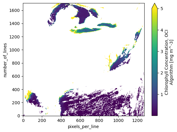
Let’s do a quick plot of the chlor_a variable.
artist = dataset["chlor_a"].plot(vmax=5)
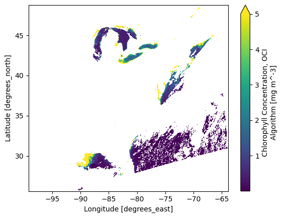
Let’s plot with latitude and longitude so we can project the data onto a grid.
dataset = dataset.set_coords(("longitude", "latitude"))
plot = dataset["chlor_a"].plot(x="longitude", y="latitude", cmap="viridis", vmax=5)
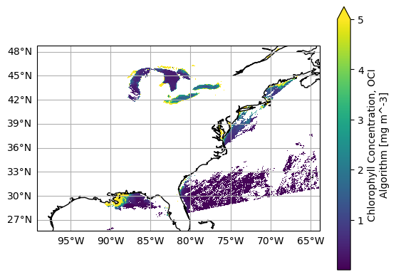
And if we want to get fancy, we can add the coastline.
fig = plt.figure()
ax = plt.axes(projection=ccrs.PlateCarree())
ax.coastlines()
ax.gridlines(draw_labels={"left": "y", "bottom": "x"})
plot = dataset["chlor_a"].plot(x="longitude", y="latitude", cmap="viridis", vmax=5, ax=ax)
5. Open L3M Data#
Let’s use earthaccess to open some L3 mapped chlorophyll a granules. We will use a new search filter available in earthaccess.search_data: the granule_name argument accepts strings with the “*” wildcard. We need this to distinguish daily (“DAY”) from eight-day (“8D”) composites, as well as to get the 0.1 degree resolution projections.
tspan = ("2024-04-12", "2024-04-24")

results = earthaccess.search_data(
    short_name="PACE_OCI_L3M_CHL_NRT",
    temporal=tspan,
    granule_name="*.DAY.*.0p1deg.*",
)

paths = earthaccess.open(results)
Let’s open the first file using xarray.
dataset = xr.open_dataset(paths[0])
dataset
<xarray.Dataset> Size: 26MB
Dimensions:  (lat: 1800, lon: 3600, rgb: 3, eightbitcolor: 256)
Coordinates:
  * lat      (lat) float32 7kB 89.95 89.85 89.75 89.65 ... -89.75 -89.85 -89.95
  * lon      (lon) float32 14kB -179.9 -179.9 -179.8 ... 179.8 179.9 180.0
Dimensions without coordinates: rgb, eightbitcolor
Data variables:
    chlor_a  (lat, lon) float32 26MB ...
    palette  (rgb, eightbitcolor) uint8 768B ...
Attributes: (12/64)
    product_name:                      PACE_OCI.20240412.L3m.DAY.CHL.V2_0.chl...
    instrument:                        OCI
    title:                             OCI Level-3 Standard Mapped Image
    project:                           Ocean Biology Processing Group (NASA/G...
    platform:                          PACE
    source:                            satellite observations from OCI-PACE
    ...                                ...
    identifier_product_doi:            10.5067/PACE/OCI/L3M/CHL/2.0
    keywords:                          Earth Science > Oceans > Ocean Chemist...
    keywords_vocabulary:               NASA Global Change Master Directory (G...
    data_bins:                         771552
    data_minimum:                      0.0069892216
data_maximum: 94.097694- lat: 1800
- lon: 3600
- rgb: 3
- eightbitcolor: 256
- lat(lat)float3289.95 89.85 89.75 ... -89.85 -89.95
- long_name :
- Latitude
- units :
- degrees_north
- standard_name :
- latitude
- valid_min :
- -90.0
- valid_max :
- 90.0
array([ 89.95 , 89.85 , 89.75 , ..., -89.75 , -89.850006, -89.950005], dtype=float32) - lon(lon)float32-179.9 -179.9 ... 179.9 180.0
- long_name :
- Longitude
- units :
- degrees_east
- standard_name :
- longitude
- valid_min :
- -180.0
- valid_max :
- 180.0
array([-179.95   , -179.85   , -179.75   , ...,  179.75   ,  179.85   ,
        179.95001], dtype=float32)
- chlor_a(lat, lon)float32...
- long_name :
- Chlorophyll Concentration, OCI Algorithm
- units :
- mg m^-3
- standard_name :
- mass_concentration_of_chlorophyll_in_sea_water
- valid_min :
- 0.001
- valid_max :
- 100.0
- reference :
- Hu, C., Lee Z., and Franz, B.A. (2012). Chlorophyll-a algorithms for oligotrophic oceans: A novel approach based on three-band reflectance difference, J. Geophys. Res., 117, C01011, doi:10.1029/2011JC007395.
- display_scale :
- log
- display_min :
- 0.01
- display_max :
- 20.0
[6480000 values with dtype=float32]
- palette(rgb, eightbitcolor)uint8...
[768 values with dtype=uint8]
- latPandasIndex
PandasIndex(Index([ 89.94999694824219, 89.8499984741211, 89.75, 89.6500015258789, 89.55000305175781, 89.44999694824219, 89.3499984741211, 89.25, 89.1500015258789, 89.05000305175781, ... -89.05000305175781, -89.1500015258789, -89.25, -89.35000610351562, -89.45000457763672, -89.55000305175781, -89.6500015258789, -89.75, -89.85000610351562, -89.95000457763672], dtype='float32', name='lat', length=1800)) - lonPandasIndex
PandasIndex(Index([ -179.9499969482422, -179.85000610351562,             -179.75,
       -179.64999389648438,  -179.5500030517578,  -179.4499969482422,
       -179.35000610351562,             -179.25, -179.14999389648438,
        -179.0500030517578,
       ...
         179.0500030517578,  179.15000915527344,              179.25,
        179.35000610351562,  179.45001220703125,   179.5500030517578,
        179.65000915527344,              179.75,  179.85000610351562,
        179.95001220703125],
      dtype='float32', name='lon', length=3600))
- product_name :
- PACE_OCI.20240412.L3m.DAY.CHL.V2_0.chlor_a.0p1deg.NRT.nc
- instrument :
- OCI
- title :
- OCI Level-3 Standard Mapped Image
- project :
- Ocean Biology Processing Group (NASA/GSFC/OBPG)
- platform :
- PACE
- source :
- satellite observations from OCI-PACE
- temporal_range :
- day
- processing_version :
- 2.0
- date_created :
- 2024-07-04T16:40:01.000Z
- history :
- l3mapgen par=PACE_OCI.20240412.L3m.DAY.CHL.V2_0.chlor_a.0p1deg.NRT.nc.param
- l2_flag_names :
- ATMFAIL,LAND,HILT,HISATZEN,STRAYLIGHT,CLDICE,COCCOLITH,LOWLW,CHLWARN,CHLFAIL,NAVWARN,MAXAERITER,ATMWARN,HISOLZEN,NAVFAIL,FILTER,HIGLINT
- time_coverage_start :
- 2024-04-12T00:43:33.000Z
- time_coverage_end :
- 2024-04-13T01:28:34.000Z
- start_orbit_number :
- 0
- end_orbit_number :
- 0
- map_projection :
- Equidistant Cylindrical
- latitude_units :
- degrees_north
- longitude_units :
- degrees_east
- northernmost_latitude :
- 90.0
- southernmost_latitude :
- -90.0
- westernmost_longitude :
- -180.0
- easternmost_longitude :
- 180.0
- geospatial_lat_max :
- 90.0
- geospatial_lat_min :
- -90.0
- geospatial_lon_max :
- 180.0
- geospatial_lon_min :
- -180.0
- latitude_step :
- 0.1
- longitude_step :
- 0.1
- sw_point_latitude :
- -89.95
- sw_point_longitude :
- -179.95
- spatialResolution :
- 11.131949 km
- geospatial_lon_resolution :
- 11.131949 km
- geospatial_lat_resolution :
- 11.131949 km
- geospatial_lat_units :
- degrees_north
- geospatial_lon_units :
- degrees_east
- number_of_lines :
- 1800
- number_of_columns :
- 3600
- measure :
- Mean
- suggested_image_scaling_minimum :
- 0.01
- suggested_image_scaling_maximum :
- 20.0
- suggested_image_scaling_type :
- LOG
- suggested_image_scaling_applied :
- No
- _lastModified :
- 2024-07-04T16:40:01.000Z
- Conventions :
- CF-1.6 ACDD-1.3
- institution :
- NASA Goddard Space Flight Center, Ocean Ecology Laboratory, Ocean Biology Processing Group
- standard_name_vocabulary :
- CF Standard Name Table v36
- naming_authority :
- gov.nasa.gsfc.sci.oceandata
- id :
- 2.0/L3/PACE_OCI.20240412.L3b.DAY.CHL.V2_0.NRT.nc
- license :
- https://science.nasa.gov/earth-science/earth-science-data/data-information-policy/
- creator_name :
- NASA/GSFC/OBPG
- publisher_name :
- NASA/GSFC/OBPG
- creator_email :
- data@oceancolor.gsfc.nasa.gov
- publisher_email :
- data@oceancolor.gsfc.nasa.gov
- creator_url :
- https://oceandata.sci.gsfc.nasa.gov
- publisher_url :
- https://oceandata.sci.gsfc.nasa.gov
- processing_level :
- L3 Mapped
- cdm_data_type :
- grid
- identifier_product_doi_authority :
- http://dx.doi.org
- identifier_product_doi :
- 10.5067/PACE/OCI/L3M/CHL/2.0
- keywords :
- Earth Science > Oceans > Ocean Chemistry > Pigments > Chlorophyll; Earth Science > Oceans > Ocean Chemistry > Chlorophyll
- keywords_vocabulary :
- NASA Global Change Master Directory (GCMD) Science Keywords
- data_bins :
- 771552
- data_minimum :
- 0.0069892216
- data_maximum :
- 94.097694
Becuase the L3M variables have lat and lon coordinates, it’s possible to stack multiple granules along a new dimension that corresponds to time. Instead of xr.open_dataset, we use xr.open_mfdataset to create a single xarray.Dataset (the “mf” in open_mfdataset stands for multiple files) from an array of paths.
The paths list is sorted temporally by default, which means the shape of the paths array specifies the way we need to tile the files together into larger arrays. We specify combine=”nested” to combine the files according to the shape of the array of files (or file-like objects), even though paths is not a “nested” list in this case. The concat_dim=”date” argument generates a new dimension in the combined dataset, because “date” is not an existing dimension in the individual files.
dataset = xr.open_mfdataset(
    paths,
    combine="nested",
    concat_dim="date",
)
dataset
<xarray.Dataset> Size: 337MB
Dimensions:  (date: 13, lat: 1800, lon: 3600, rgb: 3, eightbitcolor: 256)
Coordinates:
  * lat      (lat) float32 7kB 89.95 89.85 89.75 89.65 ... -89.75 -89.85 -89.95
  * lon      (lon) float32 14kB -179.9 -179.9 -179.8 ... 179.8 179.9 180.0
Dimensions without coordinates: date, rgb, eightbitcolor
Data variables:
    chlor_a  (date, lat, lon) float32 337MB dask.array<chunksize=(1, 512, 1024), meta=np.ndarray>
    palette  (date, rgb, eightbitcolor) uint8 10kB dask.array<chunksize=(1, 3, 256), meta=np.ndarray>
Attributes: (12/64)
    product_name:                      PACE_OCI.20240412.L3m.DAY.CHL.V2_0.chl...
    instrument:                        OCI
    title:                             OCI Level-3 Standard Mapped Image
    project:                           Ocean Biology Processing Group (NASA/G...
    platform:                          PACE
    source:                            satellite observations from OCI-PACE
    ...                                ...
    identifier_product_doi:            10.5067/PACE/OCI/L3M/CHL/2.0
    keywords:                          Earth Science > Oceans > Ocean Chemist...
    keywords_vocabulary:               NASA Global Change Master Directory (G...
    data_bins:                         771552
    data_minimum:                      0.0069892216
data_maximum: 94.097694- date: 13
- lat: 1800
- lon: 3600
- rgb: 3
- eightbitcolor: 256
- lat(lat)float3289.95 89.85 89.75 ... -89.85 -89.95
- long_name :
- Latitude
- units :
- degrees_north
- standard_name :
- latitude
- valid_min :
- -90.0
- valid_max :
- 90.0
array([ 89.95 , 89.85 , 89.75 , ..., -89.75 , -89.850006, -89.950005], dtype=float32) - lon(lon)float32-179.9 -179.9 ... 179.9 180.0
- long_name :
- Longitude
- units :
- degrees_east
- standard_name :
- longitude
- valid_min :
- -180.0
- valid_max :
- 180.0
array([-179.95   , -179.85   , -179.75   , ...,  179.75   ,  179.85   ,
        179.95001], dtype=float32)
- chlor_a(date, lat, lon)float32dask.array<chunksize=(1, 512, 1024), meta=np.ndarray>
- long_name :
- Chlorophyll Concentration, OCI Algorithm
- units :
- mg m^-3
- standard_name :
- mass_concentration_of_chlorophyll_in_sea_water
- valid_min :
- 0.001
- valid_max :
- 100.0
- reference :
- Hu, C., Lee Z., and Franz, B.A. (2012). Chlorophyll-a algorithms for oligotrophic oceans: A novel approach based on three-band reflectance difference, J. Geophys. Res., 117, C01011, doi:10.1029/2011JC007395.
- display_scale :
- log
- display_min :
- 0.01
- display_max :
- 20.0
Array Chunk Bytes 321.35 MiB 2.00 MiB Shape (13, 1800, 3600) (1, 512, 1024) Dask graph 208 chunks in 40 graph layers Data type float32 numpy.ndarray - palette(date, rgb, eightbitcolor)uint8dask.array<chunksize=(1, 3, 256), meta=np.ndarray>
Array Chunk Bytes 9.75 kiB 768 B Shape (13, 3, 256) (1, 3, 256) Dask graph 13 chunks in 40 graph layers Data type uint8 numpy.ndarray
- latPandasIndex
PandasIndex(Index([ 89.94999694824219, 89.8499984741211, 89.75, 89.6500015258789, 89.55000305175781, 89.44999694824219, 89.3499984741211, 89.25, 89.1500015258789, 89.05000305175781, ... -89.05000305175781, -89.1500015258789, -89.25, -89.35000610351562, -89.45000457763672, -89.55000305175781, -89.6500015258789, -89.75, -89.85000610351562, -89.95000457763672], dtype='float32', name='lat', length=1800)) - lonPandasIndex
PandasIndex(Index([ -179.9499969482422, -179.85000610351562,             -179.75,
       -179.64999389648438,  -179.5500030517578,  -179.4499969482422,
       -179.35000610351562,             -179.25, -179.14999389648438,
        -179.0500030517578,
       ...
         179.0500030517578,  179.15000915527344,              179.25,
        179.35000610351562,  179.45001220703125,   179.5500030517578,
        179.65000915527344,              179.75,  179.85000610351562,
        179.95001220703125],
      dtype='float32', name='lon', length=3600))
- product_name :
- PACE_OCI.20240412.L3m.DAY.CHL.V2_0.chlor_a.0p1deg.NRT.nc
- instrument :
- OCI
- title :
- OCI Level-3 Standard Mapped Image
- project :
- Ocean Biology Processing Group (NASA/GSFC/OBPG)
- platform :
- PACE
- source :
- satellite observations from OCI-PACE
- temporal_range :
- day
- processing_version :
- 2.0
- date_created :
- 2024-07-04T16:40:01.000Z
- history :
- l3mapgen par=PACE_OCI.20240412.L3m.DAY.CHL.V2_0.chlor_a.0p1deg.NRT.nc.param
- l2_flag_names :
- ATMFAIL,LAND,HILT,HISATZEN,STRAYLIGHT,CLDICE,COCCOLITH,LOWLW,CHLWARN,CHLFAIL,NAVWARN,MAXAERITER,ATMWARN,HISOLZEN,NAVFAIL,FILTER,HIGLINT
- time_coverage_start :
- 2024-04-12T00:43:33.000Z
- time_coverage_end :
- 2024-04-13T01:28:34.000Z
- start_orbit_number :
- 0
- end_orbit_number :
- 0
- map_projection :
- Equidistant Cylindrical
- latitude_units :
- degrees_north
- longitude_units :
- degrees_east
- northernmost_latitude :
- 90.0
- southernmost_latitude :
- -90.0
- westernmost_longitude :
- -180.0
- easternmost_longitude :
- 180.0
- geospatial_lat_max :
- 90.0
- geospatial_lat_min :
- -90.0
- geospatial_lon_max :
- 180.0
- geospatial_lon_min :
- -180.0
- latitude_step :
- 0.1
- longitude_step :
- 0.1
- sw_point_latitude :
- -89.95
- sw_point_longitude :
- -179.95
- spatialResolution :
- 11.131949 km
- geospatial_lon_resolution :
- 11.131949 km
- geospatial_lat_resolution :
- 11.131949 km
- geospatial_lat_units :
- degrees_north
- geospatial_lon_units :
- degrees_east
- number_of_lines :
- 1800
- number_of_columns :
- 3600
- measure :
- Mean
- suggested_image_scaling_minimum :
- 0.01
- suggested_image_scaling_maximum :
- 20.0
- suggested_image_scaling_type :
- LOG
- suggested_image_scaling_applied :
- No
- _lastModified :
- 2024-07-04T16:40:01.000Z
- Conventions :
- CF-1.6 ACDD-1.3
- institution :
- NASA Goddard Space Flight Center, Ocean Ecology Laboratory, Ocean Biology Processing Group
- standard_name_vocabulary :
- CF Standard Name Table v36
- naming_authority :
- gov.nasa.gsfc.sci.oceandata
- id :
- 2.0/L3/PACE_OCI.20240412.L3b.DAY.CHL.V2_0.NRT.nc
- license :
- https://science.nasa.gov/earth-science/earth-science-data/data-information-policy/
- creator_name :
- NASA/GSFC/OBPG
- publisher_name :
- NASA/GSFC/OBPG
- creator_email :
- data@oceancolor.gsfc.nasa.gov
- publisher_email :
- data@oceancolor.gsfc.nasa.gov
- creator_url :
- https://oceandata.sci.gsfc.nasa.gov
- publisher_url :
- https://oceandata.sci.gsfc.nasa.gov
- processing_level :
- L3 Mapped
- cdm_data_type :
- grid
- identifier_product_doi_authority :
- http://dx.doi.org
- identifier_product_doi :
- 10.5067/PACE/OCI/L3M/CHL/2.0
- keywords :
- Earth Science > Oceans > Ocean Chemistry > Pigments > Chlorophyll; Earth Science > Oceans > Ocean Chemistry > Chlorophyll
- keywords_vocabulary :
- NASA Global Change Master Directory (GCMD) Science Keywords
- data_bins :
- 771552
- data_minimum :
- 0.0069892216
- data_maximum :
- 94.097694
A common reason to generate a single dataset from multiple, daily images is to create a composite. Compare the map from a single day …
chla = np.log10(dataset["chlor_a"])
chla.attrs.update(
    {
        "units": f'lg({dataset["chlor_a"].attrs["units"]})',
    }
)
plot = chla.sel({"date": 0}).plot(aspect=2, size=4, cmap="GnBu_r")
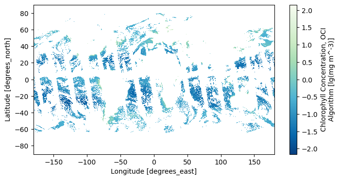
… to a map of average values, skipping “NaN” values that result from clouds.
chla_avg = chla.mean("date")
chla_avg.attrs.update(
    {
        "long_name": chla.attrs["long_name"],
        "units": f'lg({chla.attrs["units"]})',
    }
)
plot = chla_avg.plot(aspect=2, size=4, cmap="GnBu_r")
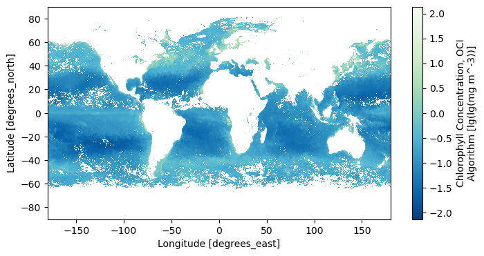
6. Download Data#
Let’s go ahead and download a couple granules.
Let’s look at the earthaccess.download function, which is used
to copy files onto a filesystem local to the machine executing the
code. For this function, provide the output of
earthaccess.search_data along with a directory where earthaccess will store downloaded granules.
Even if you only want to read a slice of the data, and downloading
seems unncessary, if you use earthaccess.open while not running on a remote host with direct access to the NASA Earthdata Cloud,
performance will be very poor. This is not a problem with “the
cloud” or with earthaccess, it has to do with the data format and may soon be resolved.
results = earthaccess.search_data(
    short_name="PACE_OCI_L2_BGC_NRT",
    temporal=tspan,
    bounding_box=bbox,
    cloud_cover=clouds,
)
The paths list now contains paths to actual files on the local
filesystem.
paths = earthaccess.download(results, local_path="data")
paths
[PosixPath('data/PACE_OCI.20240413T175656.L2.OC_BGC.V2_0.NRT.nc'),
 PosixPath('data/PACE_OCI.20240414T183158.L2.OC_BGC.V2_0.NRT.nc'),
 PosixPath('data/PACE_OCI.20240419T180521.L2.OC_BGC.V2_0.NRT.nc'),
 PosixPath('data/PACE_OCI.20240422T181158.L2.OC_BGC.V2_0.NRT.nc'),
 PosixPath('data/PACE_OCI.20240424T174337.L2.OC_BGC.V2_0.NRT.nc')]
We can open up that locally saved file using xarray as well.
open_datatree(paths[0])
<xarray.DatasetView> Size: 0B
Dimensions:  ()
Data variables:
    *empty*
Attributes: (12/45)
    title:                             OCI Level-2 Data BGC
    product_name:                      PACE_OCI.20240413T175656.L2.OC_BGC.V2_...
    processing_version:                2.0
    history:                           l2gen par=/data2/sdpsoper/vdc/vpu21/wo...
    instrument:                        OCI
    platform:                          PACE
    ...                                ...
    geospatial_lon_max:                -65.40468
    geospatial_lon_min:                -103.36526
    startDirection:                    Ascending
    endDirection:                      Ascending
    day_night_flag:                    Day
earth_sun_distance_correction: 0.9942150712013245<xarray.DatasetView> Size: 11kB Dimensions: (number_of_bands: 286, number_of_reflective_bands: 286) Dimensions without coordinates: number_of_bands, number_of_reflective_bands Data variables: wavelength (number_of_bands) float64 2kB ... vcal_gain (number_of_reflective_bands) float32 1kB ... vcal_offset (number_of_reflective_bands) float32 1kB ... F0 (number_of_reflective_bands) float32 1kB ... aw (number_of_reflective_bands) float32 1kB ... bbw (number_of_reflective_bands) float32 1kB ... k_oz (number_of_reflective_bands) float32 1kB ... k_no2 (number_of_reflective_bands) float32 1kB ... Tau_r (number_of_reflective_bands) float32 1kB ...sensor_band_parameters- number_of_bands: 286
- number_of_reflective_bands: 286
- wavelength(number_of_bands)float64...
- long_name :
- wavelengths
- units :
- nm
- valid_min :
- 0
- valid_max :
- 20000
[286 values with dtype=float64]
- vcal_gain(number_of_reflective_bands)float32...
- long_name :
- Vicarious Calibration Gain
- valid_min :
- 0.0
- valid_max :
- 2.0
[286 values with dtype=float32]
- vcal_offset(number_of_reflective_bands)float32...
- long_name :
- Vicarious Calibration Offset
- units :
- mW cm^-2 um^-1 sr^-1
- valid_min :
- 0.0
- valid_max :
- 10.0
[286 values with dtype=float32]
- F0(number_of_reflective_bands)float32...
- long_name :
- Mean Solar Flux
- units :
- W m^-2 um^-1
- valid_min :
- 0.0
- valid_max :
- 250.0
[286 values with dtype=float32]
- aw(number_of_reflective_bands)float32...
- long_name :
- Band-pass averaged absorption coefficient for seawater
- units :
- m^-1
- standard_name :
- volume_absorption_coefficient_of_radiative_flux_in_sea_water
- valid_min :
- 1e-04
- valid_max :
- 5.0
- reference :
- Pope, R.M. and Fry, E.S., 1997, "Absorption spectrum (380-700 nm) of pure water. II. Integrating cavity measurements," Appl. Opt.,36, 8710-8723.; Kou, L., Labrie, D., Chylek, P., 1993, "Refractive indices of water and ice in the 0.65-2.5 m spectral range," Appl. Opt.,32, 3531-3540 (1993).
[286 values with dtype=float32]
- bbw(number_of_reflective_bands)float32...
- long_name :
- Band-pass averaged backscattering coefficient for seawater
- units :
- m^-1
- standard_name :
- volume_backwards_scattering_coefficient_of_radiative_flux_in_sea_water
- valid_min :
- 5e-06
- valid_max :
- 1.0
- reference :
- Zhang, X., Hu, L., and He, M.-X. (2009). Scattering by pure seawater: effect of salinity, Opt. Express 17(7)
- comment :
- These are nominal values for a salinity of 38.4 at 20 degrees C. The bbw values used in the processing are corrected for temperature and salinity on a per pixel basis.
[286 values with dtype=float32]
- k_oz(number_of_reflective_bands)float32...
- long_name :
- Ozone Absorption cross-sections
- units :
- cm^-1
- valid_min :
- 0.0
- valid_max :
- 0.1
- reference :
- Anderson, S.M., Morton, J., and Mauersberger, K.. "Near-infrared absorption spectra of 16O3 and 18O3: Adiabatic energy of the 1A2 state?." The Journal of Chemical Physics 93.6 (1990): 3826-3832.; Anderson, Stuart M., Maeder, J., and Mauersberger, K. "Effect of isotopic substitution on the visible absorption spectrum of ozone." The Journal of chemical physics 94.10 (1991): 6351-6357; http://dx.doi.org/10.1029/92GL00780; http://dx.doi.org/10.1029/93GL01765; http://dx.doi.org/10.1029/93GL02311
- comment :
- Computed at 229.15K with code provided by E.P.Shettle, NRL, Washington, DC; Based on the measurements of: S.Anderson et al. and J. Burkholder and Talukdar (1994)
[286 values with dtype=float32]
- k_no2(number_of_reflective_bands)float32...
- long_name :
- NO2 Absorption cross-sections
- units :
- cm^2 molecule^-1
- valid_min :
- 0.0
- valid_max :
- 0.1
- reference :
- K. Bogumil, et al., "Measurements of molecular absorption spectra with the SCIAMACHY pre-flight model: Instrument characterization and reference data for atmospheric remote sensing in the 230-2380 nm region," J. Photochem. Photobiol. A.: Photochem. 157, 167-184 (2003).; W. Schneider,et al., "Absorption cross-sections of NO2 in the UV and visible region (200 - 700 nm) at 298 K", J. Photochem. Photobiol. 40, 195-217 (1987)
[286 values with dtype=float32]
- Tau_r(number_of_reflective_bands)float32...
- long_name :
- Rayleigh Optical Thickness
- valid_min :
- 0.0
- valid_max :
- 0.5
- reference :
- Bodhaine, B.A., Wood, N.B, Dutton, E.G., Slusser, J.R. (1999). On Rayleigh Optical Depth Calculations, J. Atmos. Ocean Tech., 16, 1854-1861.
[286 values with dtype=float32]
<xarray.DatasetView> Size: 103kB Dimensions: (number_of_lines: 1710) Dimensions without coordinates: number_of_lines Data variables: year (number_of_lines) float64 14kB ... day (number_of_lines) timedelta64[ns] 14kB ... msec (number_of_lines) timedelta64[ns] 14kB ... detnum (number_of_lines) float32 7kB ... mside (number_of_lines) float32 7kB ... slon (number_of_lines) float32 7kB ... clon (number_of_lines) float32 7kB ... elon (number_of_lines) float32 7kB ... slat (number_of_lines) float32 7kB ... clat (number_of_lines) float32 7kB ... elat (number_of_lines) float32 7kB ... csol_z (number_of_lines) float32 7kB ...scan_line_attributes- number_of_lines: 1710
- year(number_of_lines)float64...
- long_name :
- Scan year
- units :
- years
- valid_min :
- 1900
- valid_max :
- 2100
[1710 values with dtype=float64]
- day(number_of_lines)timedelta64[ns]...
- long_name :
- Scan day of year
- valid_min :
- 0
- valid_max :
- 366
[1710 values with dtype=timedelta64[ns]]
- msec(number_of_lines)timedelta64[ns]...
- long_name :
- Scan time, milliseconds of day
- valid_min :
- 0
- valid_max :
- 86400000
[1710 values with dtype=timedelta64[ns]]
- detnum(number_of_lines)float32...
- long_name :
- Detector Number (zero-based)
- valid_min :
- 0
- valid_max :
- 25
[1710 values with dtype=float32]
- mside(number_of_lines)float32...
- long_name :
- Mirror Side (zero-based)
- valid_min :
- 0
- valid_max :
- 1
[1710 values with dtype=float32]
- slon(number_of_lines)float32...
- long_name :
- Starting Longitude
- units :
- degrees_east
- standard_name :
- longitude
- valid_min :
- -180.0
- valid_max :
- 180.0
[1710 values with dtype=float32]
- clon(number_of_lines)float32...
- long_name :
- Center Longitude
- units :
- degrees_east
- standard_name :
- longitude
- valid_min :
- -180.0
- valid_max :
- 180.0
[1710 values with dtype=float32]
- elon(number_of_lines)float32...
- long_name :
- Ending Longitude
- units :
- degrees_east
- standard_name :
- longitude
- valid_min :
- -180.0
- valid_max :
- 180.0
[1710 values with dtype=float32]
- slat(number_of_lines)float32...
- long_name :
- Starting Latitude
- units :
- degrees_north
- standard_name :
- latitude
- valid_min :
- -90.0
- valid_max :
- 90.0
[1710 values with dtype=float32]
- clat(number_of_lines)float32...
- long_name :
- Center Latitude
- units :
- degrees_north
- standard_name :
- latitude
- valid_min :
- -90.0
- valid_max :
- 90.0
[1710 values with dtype=float32]
- elat(number_of_lines)float32...
- long_name :
- Ending Latitude
- units :
- degrees_north
- standard_name :
- latitude
- valid_min :
- -90.0
- valid_max :
- 90.0
[1710 values with dtype=float32]
- csol_z(number_of_lines)float32...
- long_name :
- Center Solar Zenith Angle
- units :
- degree
- valid_min :
- -90.0
- valid_max :
- 90.0
[1710 values with dtype=float32]
<xarray.DatasetView> Size: 52MB Dimensions: (number_of_lines: 1710, pixels_per_line: 1272) Dimensions without coordinates: number_of_lines, pixels_per_line Data variables: chlor_a (number_of_lines, pixels_per_line) float32 9MB ... carbon_phyto (number_of_lines, pixels_per_line) float32 9MB ... poc (number_of_lines, pixels_per_line) float32 9MB ... chlor_a_unc (number_of_lines, pixels_per_line) float32 9MB ... carbon_phyto_unc (number_of_lines, pixels_per_line) float32 9MB ... l2_flags (number_of_lines, pixels_per_line) int32 9MB ...geophysical_data- number_of_lines: 1710
- pixels_per_line: 1272
- chlor_a(number_of_lines, pixels_per_line)float32...
- long_name :
- Chlorophyll Concentration, OCI Algorithm
- units :
- mg m^-3
- standard_name :
- mass_concentration_of_chlorophyll_in_sea_water
- valid_min :
- 0.001
- valid_max :
- 100.0
- reference :
- Hu, C., Lee Z., and Franz, B.A. (2012). Chlorophyll-a algorithms for oligotrophic oceans: A novel approach based on three-band reflectance difference, J. Geophys. Res., 117, C01011, doi:10.1029/2011JC007395.
[2175120 values with dtype=float32]
- carbon_phyto(number_of_lines, pixels_per_line)float32...
- long_name :
- Phytoplankton Carbon
- units :
- mg m^-3
- valid_min :
- 0.0
- valid_max :
- 1000.0
- reference :
- Graff, J.R., Westberry, T.K., Milligan, A.J., Brown, M.B., Dall'Olmo, G., Dongen-Vogels, V.v., Reifel, K.M., and Behrenfeld, M.J. (2015). Analytical phytoplankton carbon measurements spanning diverse ecosystems. Deep Sea Research Part I: Oceanographic Research Papers, 102, 16-25
[2175120 values with dtype=float32]
- poc(number_of_lines, pixels_per_line)float32...
- long_name :
- Particulate Organic Carbon, D. Stramski, 2022 (hybrid version)
- units :
- mg m^-3
- valid_min :
- -32000
- valid_max :
- -22000
- reference :
- Stramski, D., et al. "Ocean color algorithms to estimate the concentration of particulate organic carbon in surface waters of the global ocean in support of a long-term data record from multiple satellite missions." Remote Sensing of Environment 269 (2022)
[2175120 values with dtype=float32]
- chlor_a_unc(number_of_lines, pixels_per_line)float32...
- long_name :
- Uncertainty in chlorophyll a concentration
- units :
- mg m^-3
- standard_name :
- chlorophyll_concentration_in_sea_water standard_error
- valid_min :
- 0.001
- valid_max :
- 100.0
[2175120 values with dtype=float32]
- carbon_phyto_unc(number_of_lines, pixels_per_line)float32...
- long_name :
- Phytoplankton Carbon standard uncertainty
- units :
- mg m^-3
- valid_min :
- 0.0
- valid_max :
- 1000.0
- reference :
- Graff, J.R., Westberry, T.K., Milligan, A.J., Brown, M.B., Dall'Olmo, G., Dongen-Vogels, V.v., Reifel, K.M., and Behrenfeld, M.J. (2015). Analytical phytoplankton carbon measurements spanning diverse ecosystems. Deep Sea Research Part I: Oceanographic Research Papers, 102, 16-25
[2175120 values with dtype=float32]
- l2_flags(number_of_lines, pixels_per_line)int32...
- long_name :
- Level-2 Processing Flags
- valid_min :
- -2147483648
- valid_max :
- 2147483647
- flag_masks :
- [ 1 2 4 8 16 32 64 128 256 512 1024 2048 4096 8192 16384 32768 65536 131072 262144 524288 1048576 2097152 4194304 8388608 16777216 33554432 67108864 134217728 268435456 536870912 1073741824 -2147483648]
- flag_meanings :
- ATMFAIL LAND PRODWARN HIGLINT HILT HISATZEN COASTZ SPARE STRAYLIGHT CLDICE COCCOLITH TURBIDW HISOLZEN SPARE LOWLW CHLFAIL NAVWARN ABSAER SPARE MAXAERITER MODGLINT CHLWARN ATMWARN SPARE SEAICE NAVFAIL FILTER SPARE BOWTIEDEL HIPOL PRODFAIL SPARE
[2175120 values with dtype=int32]
<xarray.DatasetView> Size: 17MB Dimensions: (number_of_lines: 1710, pixels_per_line: 1272) Dimensions without coordinates: number_of_lines, pixels_per_line Data variables: longitude (number_of_lines, pixels_per_line) float32 9MB ... latitude (number_of_lines, pixels_per_line) float32 9MB ... tilt (number_of_lines) float32 7kB ... Attributes: gringpointlongitude: [ -93.578735 -65.40468 -66.24995 -103.36526 ] gringpointlatitude: [30.214327 35.672337 53.449913 47.069923] gringpointsequence: [1 2 3 4]navigation_data- number_of_lines: 1710
- pixels_per_line: 1272
- longitude(number_of_lines, pixels_per_line)float32...
- long_name :
- Longitude
- units :
- degrees_east
- standard_name :
- longitude
- valid_min :
- -180.0
- valid_max :
- 180.0
[2175120 values with dtype=float32]
- latitude(number_of_lines, pixels_per_line)float32...
- long_name :
- Latitude
- units :
- degrees_north
- standard_name :
- latitude
- valid_min :
- -90.0
- valid_max :
- 90.0
[2175120 values with dtype=float32]
- tilt(number_of_lines)float32...
- long_name :
- Sensor tilt angle
- units :
- degree
- valid_min :
- -25.0
- valid_max :
- 25.0
[1710 values with dtype=float32]
- gringpointlongitude :
- [ -93.578735 -65.40468 -66.24995 -103.36526 ]
- gringpointlatitude :
- [30.214327 35.672337 53.449913 47.069923]
- gringpointsequence :
- [1 2 3 4]
<xarray.DatasetView> Size: 0B Dimensions: () Data variables: *empty* Attributes: software_name: l2gen software_version: 9.7.0-V2024.0 input_sources: PACE_OCI.20240413T175656.L1B.V2.nc,GMAO_MERRA2.2024041... calibration_data: mask_names: ATMFAIL,LAND,CLDICE,HILTprocessing_control<xarray.DatasetView> Size: 0B Dimensions: () Data variables: *empty* Attributes: (12/248) ifile: PACE_OCI.20240413T175656.L1B.V2.nc ofile: PACE_OCI.20240413T175656.L2.OC_BGC.V2_0.NRT.nc l2prod: chlor_a carbon_phyto poc chlor_a_unc carbon_phyto_unc oformat: netCDF4 oformat_depth: 8bit fqfile: $OCDATAROOT/common/morel_fq.nc ... ... spixl: 1 epixl: -1 dpixl: 1 sline: 1 eline: -1 dline: 1input_parameters- ifile :
- PACE_OCI.20240413T175656.L1B.V2.nc
- ofile :
- PACE_OCI.20240413T175656.L2.OC_BGC.V2_0.NRT.nc
- l2prod :
- chlor_a carbon_phyto poc chlor_a_unc carbon_phyto_unc
- oformat :
- netCDF4
- oformat_depth :
- 8bit
- fqfile :
- $OCDATAROOT/common/morel_fq.nc
- parfile :
- geofile :
- gmpfile :
- metafile :
- PACE_OCI.20240413T175656.L2.OC_BGC.V2_0.NRT.nc.meta
- suite :
- BGC
- mode :
- 0
- deflate :
- 4
- proc_ocean :
- 1
- proc_land :
- 1
- proc_cloud :
- 0
- proc_uncertainty :
- 1
- proc_sst :
- 0
- atmocor :
- 1
- seawater_opt :
- 1
- aermodfile :
- $OCDATAROOT/oci/aerosol/aerosol_oci
- uncertaintyfile :
- $OCDATAROOT/oci/uncertainty.nc
- aer_opt :
- -18
- aer_wave_short :
- 751
- aer_wave_long :
- 870
- aer_wave_base :
- 870
- aer_swir_short :
- -1
- aer_swir_long :
- -1
- aer_rrs_short :
- -1.00000
- aer_rrs_long :
- -1.00000
- aer_angstrom :
- -999.00000
- aer_iter_max :
- 10
- brdf_opt :
- 7
- gas_opt :
- 491
- atrem_opt :
- 0
- atrem_full :
- 0
- atrem_geom :
- 0
- atrem_model :
- 0
- atrem_splitpaths :
- 0
- iop_opt :
- 0
- cphyt_opt :
- 1
- gsm_opt :
- 0
- gsm_fit :
- 0
- gsm_adg_s :
- 0.02061
- gsm_bbp_s :
- 1.03373
- gsm_aphw :
- 412.00000, 443.00000, 490.00000, 510.00000, 555.00000, 670.00000, -1.00000, -1.00000, -1.00000, -1.00000, -1.00000, -1.00000, -1.00000, -1.00000, -1.00000, -1.00000, -1.00000, -1.00000, -1.00000, -1.00000, -1.00000, -1.00000, -1.00000, -1.00000, -1.00000, -1.00000, -1.00000, -1.00000, -1.00000, -1.00000, -1.00000, -1.00000, -1.00000, -1.00000, -1.00000, -1.00000, -1.00000, -1.00000, -1.00000, -1.00000, -1.00000, -1.00000, -1.00000, -1.00000, -1.00000, -1.00000, -1.00000, -1.00000, -1.00000, -1.00000, -1.00000, -1.00000, -1.00000, -1.00000, -1.00000, -1.00000, -1.00000, -1.00000, -1.00000, -1.00000, -1.00000, -1.00000, -1.00000, -1.00000, -1.00000, -1.00000, -1.00000, -1.00000, -1.00000, -1.00000, -1.00000, -1.00000, -1.00000, -1.00000, -1.00000, -1.00000, -1.00000, -1.00000, -1.00000, -1.00000, -1.00000, -1.00000, -1.00000, -1.00000, -1.00000, -1.00000, -1.00000, -1.00000, -1.00000, -1.00000, -1.00000, -1.00000, -1.00000, -1.00000, -1.00000, -1.00000, -1.00000, -1.00000, -1.00000, -1.00000, -1.00000, -1.00000, -1.00000, -1.00000, -1.00000, -1.00000, -1.00000, -1.00000, -1.00000, -1.00000, -1.00000, -1.00000, -1.00000, -1.00000, -1.00000, -1.00000, -1.00000, -1.00000, -1.00000, -1.00000, -1.00000, -1.00000, -1.00000, -1.00000, -1.00000, -1.00000, -1.00000, -1.00000, -1.00000, -1.00000, -1.00000, -1.00000, -1.00000, -1.00000, -1.00000, -1.00000, -1.00000, -1.00000, -1.00000, -1.00000, -1.00000, -1.00000, -1.00000, -1.00000, -1.00000, -1.00000, -1.00000, -1.00000, -1.00000, -1.00000, -1.00000, -1.00000, -1.00000, -1.00000, -1.00000, -1.00000, -1.00000, -1.00000, -1.00000, -1.00000, -1.00000, -1.00000, -1.00000, -1.00000, -1.00000, -1.00000, -1.00000, -1.00000, -1.00000, -1.00000, -1.00000, -1.00000, -1.00000, -1.00000, -1.00000, -1.00000, -1.00000, -1.00000, -1.00000, -1.00000, -1.00000, -1.00000, -1.00000, -1.00000, -1.00000, -1.00000, -1.00000, -1.00000, -1.00000, -1.00000, -1.00000, -1.00000, -1.00000, -1.00000, -1.00000, -1.00000, -1.00000, -1.00000, -1.00000, -1.00000, -1.00000, -1.00000, -1.00000, -1.00000, -1.00000, -1.00000, -1.00000, -1.00000, -1.00000, -1.00000, -1.00000, -1.00000, -1.00000, -1.00000, -1.00000, -1.00000, -1.00000, -1.00000, -1.00000, -1.00000, -1.00000, -1.00000, -1.00000, -1.00000, -1.00000, -1.00000, -1.00000, -1.00000, -1.00000, -1.00000, -1.00000, -1.00000, -1.00000, -1.00000, -1.00000, -1.00000, -1.00000, -1.00000, -1.00000, -1.00000, -1.00000, -1.00000, -1.00000, -1.00000, -1.00000, -1.00000, -1.00000, -1.00000, -1.00000, -1.00000, -1.00000, -1.00000, -1.00000, -1.00000, -1.00000, -1.00000, -1.00000, -1.00000, -1.00000, -1.00000, -1.00000, -1.00000, -1.00000, -1.00000, -1.00000, -1.00000, -1.00000, -1.00000, -1.00000, -1.00000, -1.00000, -1.00000, -1.00000, -1.00000, -1.00000, -1.00000, -1.00000, -1.00000, -1.00000, -1.00000, -1.00000, -1.00000, -1.00000, -1.00000, -1.00000, -1.00000
- gsm_aphs :
- 0.00665, 0.05582, 0.02055, 0.01910, 0.01015, 0.01424, -1.00000, -1.00000, -1.00000, -1.00000, -1.00000, -1.00000, -1.00000, -1.00000, -1.00000, -1.00000, -1.00000, -1.00000, -1.00000, -1.00000, -1.00000, -1.00000, -1.00000, -1.00000, -1.00000, -1.00000, -1.00000, -1.00000, -1.00000, -1.00000, -1.00000, -1.00000, -1.00000, -1.00000, -1.00000, -1.00000, -1.00000, -1.00000, -1.00000, -1.00000, -1.00000, -1.00000, -1.00000, -1.00000, -1.00000, -1.00000, -1.00000, -1.00000, -1.00000, -1.00000, -1.00000, -1.00000, -1.00000, -1.00000, -1.00000, -1.00000, -1.00000, -1.00000, -1.00000, -1.00000, -1.00000, -1.00000, -1.00000, -1.00000, -1.00000, -1.00000, -1.00000, -1.00000, -1.00000, -1.00000, -1.00000, -1.00000, -1.00000, -1.00000, -1.00000, -1.00000, -1.00000, -1.00000, -1.00000, -1.00000, -1.00000, -1.00000, -1.00000, -1.00000, -1.00000, -1.00000, -1.00000, -1.00000, -1.00000, -1.00000, -1.00000, -1.00000, -1.00000, -1.00000, -1.00000, -1.00000, -1.00000, -1.00000, -1.00000, -1.00000, -1.00000, -1.00000, -1.00000, -1.00000, -1.00000, -1.00000, -1.00000, -1.00000, -1.00000, -1.00000, -1.00000, -1.00000, -1.00000, -1.00000, -1.00000, -1.00000, -1.00000, -1.00000, -1.00000, -1.00000, -1.00000, -1.00000, -1.00000, -1.00000, -1.00000, -1.00000, -1.00000, -1.00000, -1.00000, -1.00000, -1.00000, -1.00000, -1.00000, -1.00000, -1.00000, -1.00000, -1.00000, -1.00000, -1.00000, -1.00000, -1.00000, -1.00000, -1.00000, -1.00000, -1.00000, -1.00000, -1.00000, -1.00000, -1.00000, -1.00000, -1.00000, -1.00000, -1.00000, -1.00000, -1.00000, -1.00000, -1.00000, -1.00000, -1.00000, -1.00000, -1.00000, -1.00000, -1.00000, -1.00000, -1.00000, -1.00000, -1.00000, -1.00000, -1.00000, -1.00000, -1.00000, -1.00000, -1.00000, -1.00000, -1.00000, -1.00000, -1.00000, -1.00000, -1.00000, -1.00000, -1.00000, -1.00000, -1.00000, -1.00000, -1.00000, -1.00000, -1.00000, -1.00000, -1.00000, -1.00000, -1.00000, -1.00000, -1.00000, -1.00000, -1.00000, -1.00000, -1.00000, -1.00000, -1.00000, -1.00000, -1.00000, -1.00000, -1.00000, -1.00000, -1.00000, -1.00000, -1.00000, -1.00000, -1.00000, -1.00000, -1.00000, -1.00000, -1.00000, -1.00000, -1.00000, -1.00000, -1.00000, -1.00000, -1.00000, -1.00000, -1.00000, -1.00000, -1.00000, -1.00000, -1.00000, -1.00000, -1.00000, -1.00000, -1.00000, -1.00000, -1.00000, -1.00000, -1.00000, -1.00000, -1.00000, -1.00000, -1.00000, -1.00000, -1.00000, -1.00000, -1.00000, -1.00000, -1.00000, -1.00000, -1.00000, -1.00000, -1.00000, -1.00000, -1.00000, -1.00000, -1.00000, -1.00000, -1.00000, -1.00000, -1.00000, -1.00000, -1.00000, -1.00000, -1.00000, -1.00000, -1.00000, -1.00000, -1.00000, -1.00000, -1.00000, -1.00000, -1.00000, -1.00000, -1.00000, -1.00000, -1.00000, -1.00000, -1.00000, -1.00000, -1.00000, -1.00000, -1.00000, -1.00000, -1.00000, -1.00000, -1.00000, -1.00000, -1.00000, -1.00000, -1.00000, -1.00000
- qaa_adg_s :
- 0.01500
- qaa_wave :
- 410, 440, 490, 555, 670
- giop_maxiter :
- 50
- giop_fit_opt :
- 1
- giop_aph_opt :
- 2
- giop_acdom_opt :
- 1
- giop_anap_opt :
- 1
- giop_adg_opt :
- 1
- giop_bbp_opt :
- 3
- giop_bbnap_opt :
- 1
- giop_bbph_opt :
- 1
- giop_rrs_opt :
- 0
- giop_rrs_diff :
- 0.33000
- giop_aph_file :
- $OCDATAROOT/common/aph_default.txt
- giop_uaph_file :
- $OCDATAROOT/common/aph_unc_default.txt
- giop_aph_s :
- -1000.00000
- giop_adg_file :
- $OCDATAROOT/common/adg_default.txt
- giop_uadg_file :
- $OCDATAROOT/common/adg_unc_default.txt
- giop_adg_s :
- 0.01800
- giop_uadg_s :
- 0.00000
- giop_bbp_file :
- $OCDATAROOT/common/bbp_default.txt
- giop_bbp_s :
- -1000.00000
- giop_ubbp_s :
- 0.00000
- giop_acdom_file :
- giop_uacdom_file :
- giop_anap_file :
- giop_uanap_file :
- giop_bbph_file :
- giop_ubbph_file :
- giop_bbnap_file :
- giop_ubbnap_file :
- giop_grd :
- 0.09490, 0.07940
- giop_wave :
- 413.0, 442.0, 490.0, 510.0, 555.0, 670.0, -1.0, -1.0, -1.0, -1.0, -1.0, -1.0, -1.0, -1.0, -1.0, -1.0, -1.0, -1.0, -1.0, -1.0, -1.0, -1.0, -1.0, -1.0, -1.0, -1.0, -1.0, -1.0, -1.0, -1.0, -1.0, -1.0, -1.0, -1.0, -1.0, -1.0, -1.0, -1.0, -1.0, -1.0, -1.0, -1.0, -1.0, -1.0, -1.0, -1.0, -1.0, -1.0, -1.0, -1.0, -1.0, -1.0, -1.0, -1.0, -1.0, -1.0, -1.0, -1.0, -1.0, -1.0, -1.0, -1.0, -1.0, -1.0, -1.0, -1.0, -1.0, -1.0, -1.0, -1.0, -1.0, -1.0, -1.0, -1.0, -1.0, -1.0, -1.0, -1.0, -1.0, -1.0, -1.0, -1.0, -1.0, -1.0, -1.0, -1.0, -1.0, -1.0, -1.0, -1.0, -1.0, -1.0, -1.0, -1.0, -1.0, -1.0, -1.0, -1.0, -1.0, -1.0, -1.0, -1.0, -1.0, -1.0, -1.0, -1.0, -1.0, -1.0, -1.0, -1.0, -1.0, -1.0, -1.0, -1.0, -1.0, -1.0, -1.0, -1.0, -1.0, -1.0, -1.0, -1.0, -1.0, -1.0, -1.0, -1.0, -1.0, -1.0, -1.0, -1.0, -1.0, -1.0, -1.0, -1.0, -1.0, -1.0, -1.0, -1.0, -1.0, -1.0, -1.0, -1.0, -1.0, -1.0, -1.0, -1.0, -1.0, -1.0, -1.0, -1.0, -1.0, -1.0, -1.0, -1.0, -1.0, -1.0, -1.0, -1.0, -1.0, -1.0, -1.0, -1.0, -1.0, -1.0, -1.0, -1.0, -1.0, -1.0, -1.0, -1.0, -1.0, -1.0, -1.0, -1.0, -1.0, -1.0, -1.0, -1.0, -1.0, -1.0, -1.0, -1.0, -1.0, -1.0, -1.0, -1.0, -1.0, -1.0, -1.0, -1.0, -1.0, -1.0, -1.0, -1.0, -1.0, -1.0, -1.0, -1.0, -1.0, -1.0, -1.0, -1.0, -1.0, -1.0, -1.0, -1.0, -1.0, -1.0, -1.0, -1.0, -1.0, -1.0, -1.0, -1.0, -1.0, -1.0, -1.0, -1.0, -1.0, -1.0, -1.0, -1.0, -1.0, -1.0, -1.0, -1.0, -1.0, -1.0, -1.0, -1.0, -1.0, -1.0, -1.0, -1.0, -1.0, -1.0, -1.0, -1.0, -1.0, -1.0, -1.0, -1.0, -1.0, -1.0, -1.0, -1.0, -1.0, -1.0, -1.0, -1.0, -1.0, -1.0, -1.0, -1.0, -1.0, -1.0, -1.0, -1.0, -1.0, -1.0, -1.0, -1.0, -1.0, -1.0, -1.0, -1.0, -1.0, -1.0, -1.0, -1.0, -1.0, -1.0, -1.0, -1.0, -1.0, -1.0, -1.0, -1.0, -1.0, -1.0, -1.0, -1.0, -1.0, -1.0, -1.0, -1.0
- giop_rrs_unc_opt :
- 0
- giop_rrs_unc :
- -1.0, -1.0, -1.0, -1.0, -1.0, -1.0, -1.0, -1.0, -1.0, -1.0, -1.0, -1.0, -1.0, -1.0, -1.0, -1.0, -1.0, -1.0, -1.0, -1.0, -1.0, -1.0, -1.0, -1.0, -1.0, -1.0, -1.0, -1.0, -1.0, -1.0, -1.0, -1.0, -1.0, -1.0, -1.0, -1.0, -1.0, -1.0, -1.0, -1.0, -1.0, -1.0, -1.0, -1.0, -1.0, -1.0, -1.0, -1.0, -1.0, -1.0, -1.0, -1.0, -1.0, -1.0, -1.0, -1.0, -1.0, -1.0, -1.0, -1.0, -1.0, -1.0, -1.0, -1.0, -1.0, -1.0, -1.0, -1.0, -1.0, -1.0, -1.0, -1.0, -1.0, -1.0, -1.0, -1.0, -1.0, -1.0, -1.0, -1.0, -1.0, -1.0, -1.0, -1.0, -1.0, -1.0, -1.0, -1.0, -1.0, -1.0, -1.0, -1.0, -1.0, -1.0, -1.0, -1.0, -1.0, -1.0, -1.0, -1.0, -1.0, -1.0, -1.0, -1.0, -1.0, -1.0, -1.0, -1.0, -1.0, -1.0, -1.0, -1.0, -1.0, -1.0, -1.0, -1.0, -1.0, -1.0, -1.0, -1.0, -1.0, -1.0, -1.0, -1.0, -1.0, -1.0, -1.0, -1.0, -1.0, -1.0, -1.0, -1.0, -1.0, -1.0, -1.0, -1.0, -1.0, -1.0, -1.0, -1.0, -1.0, -1.0, -1.0, -1.0, -1.0, -1.0, -1.0, -1.0, -1.0, -1.0, -1.0, -1.0, -1.0, -1.0, -1.0, -1.0, -1.0, -1.0, -1.0, -1.0, -1.0, -1.0, -1.0, -1.0, -1.0, -1.0, -1.0, -1.0, -1.0, -1.0, -1.0, -1.0, -1.0, -1.0, -1.0, -1.0, -1.0, -1.0, -1.0, -1.0, -1.0, -1.0, -1.0, -1.0, -1.0, -1.0, -1.0, -1.0, -1.0, -1.0, -1.0, -1.0, -1.0, -1.0, -1.0, -1.0, -1.0, -1.0, -1.0, -1.0, -1.0, -1.0, -1.0, -1.0, -1.0, -1.0, -1.0, -1.0, -1.0, -1.0, -1.0, -1.0, -1.0, -1.0, -1.0, -1.0, -1.0, -1.0, -1.0, -1.0, -1.0, -1.0, -1.0, -1.0, -1.0, -1.0, -1.0, -1.0, -1.0, -1.0, -1.0, -1.0, -1.0, -1.0, -1.0, -1.0, -1.0, -1.0, -1.0, -1.0, -1.0, -1.0, -1.0, -1.0, -1.0, -1.0, -1.0, -1.0, -1.0, -1.0, -1.0, -1.0, -1.0, -1.0, -1.0, -1.0, -1.0, -1.0, -1.0, -1.0, -1.0, -1.0, -1.0, -1.0, -1.0, -1.0, -1.0, -1.0, -1.0, -1.0, -1.0, -1.0, -1.0, -1.0, -1.0, -1.0, -1.0, -1.0, -1.0, -1.0, -1.0, -1.0, -1.0, -1.0, -1.0, -1.0
- polfile :
- pol_opt :
- 0
- vcnnfile :
- absaer_opt :
- 2
- glint_opt :
- 1
- cirrus_opt :
- 0
- oxaband_opt :
- 2
- filter_opt :
- 1
- filter_file :
- $OCDATAROOT/oci/msl12_filter.dat
- aerfile :
- tgtfile :
- met1 :
- GMAO_MERRA2.20240413T170000.MET.nc
- met2 :
- GMAO_MERRA2.20240413T180000.MET.nc
- met3 :
- GMAO_MERRA2.20240413T190000.MET.nc
- ozone1 :
- GMAO_MERRA2.20240413T170000.MET.nc
- ozone2 :
- GMAO_MERRA2.20240413T180000.MET.nc
- ozone3 :
- GMAO_MERRA2.20240413T190000.MET.nc
- rad1 :
- rad2 :
- rad3 :
- anc_profile1 :
- anc_profile2 :
- anc_profile3 :
- anc_aerosol1 :
- GMAO_MERRA2.20240413T170000.AER.nc
- anc_aerosol2 :
- GMAO_MERRA2.20240413T180000.AER.nc
- anc_aerosol3 :
- GMAO_MERRA2.20240413T190000.AER.nc
- sfc_albedo :
- cth_albedo :
- anc_cor_file :
- $OCDATAROOT/common/anc_cor_file_28jan2014.nc
- pixel_anc_file :
- land :
- $OCDATAROOT/common/gebco_ocssw_v2020.nc
- water :
- $OCDATAROOT/common/gebco_ocssw_v2020.nc
- shallow_water_depth :
- 30.00
- demfile :
- $OCDATAROOT/common/gebco_ocssw_v2020.nc
- dem_auxfile :
- mldfile :
- $OCDATAROOT/common/mld_climatology_woa1994.hdf
- icefile :
- 20240413120000-CMC-L4_GHRSST-SSTfnd-CMC0.1deg-GLOB-v02.0-fv03.0.nc
- sstfile :
- 20240413120000-CMC-L4_GHRSST-SSTfnd-CMC0.1deg-GLOB-v02.0-fv03.0.nc
- sstreftype :
- 0
- sssfile :
- $OCDATAROOT/common/sss_climatology_woa2009.hdf
- no2file :
- $OCDATAROOT/common/no2_climatology_v2013.hdf
- alphafile :
- $OCDATAROOT/common/alpha510_climatology.hdf
- tauafile :
- $OCDATAROOT/common/taua865_climatology.hdf
- picfile :
- $OCDATAROOT/common/calcite_table-20170109.txt
- owmcfile :
- $OCDATAROOT/common/owmc_lut.hdf
- prodxmlfile :
- breflectfile :
- aerbinfile :
- naermodels :
- 80
- aermodels :
- r30f95, r30f80, r30f50, r30f30, r30f20, r30f10, r30f05, r30f02, r30f01, r30f00, r50f95, r50f80, r50f50, r50f30, r50f20, r50f10, r50f05, r50f02, r50f01, r50f00, r70f95, r70f80, r70f50, r70f30, r70f20, r70f10, r70f05, r70f02, r70f01, r70f00, r75f95, r75f80, r75f50, r75f30, r75f20, r75f10, r75f05, r75f02, r75f01, r75f00, r80f95, r80f80, r80f50, r80f30, r80f20, r80f10, r80f05, r80f02, r80f01, r80f00, r85f95, r85f80, r85f50, r85f30, r85f20, r85f10, r85f05, r85f02, r85f01, r85f00, r90f95, r90f80, r90f50, r90f30, r90f20, r90f10, r90f05, r90f02, r90f01, r90f00, r95f95, r95f80, r95f50, r95f30, r95f20, r95f10, r95f05, r95f02, r95f01, r95f00
- taua :
- 0.0000, 0.0000, 0.0000, 0.0000, 0.0000, 0.0000, 0.0000, 0.0000, 0.0000, 0.0000, 0.0000, 0.0000, 0.0000, 0.0000, 0.0000, 0.0000, 0.0000, 0.0000, 0.0000, 0.0000, 0.0000, 0.0000, 0.0000, 0.0000, 0.0000, 0.0000, 0.0000, 0.0000, 0.0000, 0.0000, 0.0000, 0.0000, 0.0000, 0.0000, 0.0000, 0.0000, 0.0000, 0.0000, 0.0000, 0.0000, 0.0000, 0.0000, 0.0000, 0.0000, 0.0000, 0.0000, 0.0000, 0.0000, 0.0000, 0.0000, 0.0000, 0.0000, 0.0000, 0.0000, 0.0000, 0.0000, 0.0000, 0.0000, 0.0000, 0.0000, 0.0000, 0.0000, 0.0000, 0.0000, 0.0000, 0.0000, 0.0000, 0.0000, 0.0000, 0.0000, 0.0000, 0.0000, 0.0000, 0.0000, 0.0000, 0.0000, 0.0000, 0.0000, 0.0000, 0.0000, 0.0000, 0.0000, 0.0000, 0.0000, 0.0000, 0.0000, 0.0000, 0.0000, 0.0000, 0.0000, 0.0000, 0.0000, 0.0000, 0.0000, 0.0000, 0.0000, 0.0000, 0.0000, 0.0000, 0.0000, 0.0000, 0.0000, 0.0000, 0.0000, 0.0000, 0.0000, 0.0000, 0.0000, 0.0000, 0.0000, 0.0000, 0.0000, 0.0000, 0.0000, 0.0000, 0.0000, 0.0000, 0.0000, 0.0000, 0.0000, 0.0000, 0.0000, 0.0000, 0.0000, 0.0000, 0.0000, 0.0000, 0.0000, 0.0000, 0.0000, 0.0000, 0.0000, 0.0000, 0.0000, 0.0000, 0.0000, 0.0000, 0.0000, 0.0000, 0.0000, 0.0000, 0.0000, 0.0000, 0.0000, 0.0000, 0.0000, 0.0000, 0.0000, 0.0000, 0.0000, 0.0000, 0.0000, 0.0000, 0.0000, 0.0000, 0.0000, 0.0000, 0.0000, 0.0000, 0.0000, 0.0000, 0.0000, 0.0000, 0.0000, 0.0000, 0.0000, 0.0000, 0.0000, 0.0000, 0.0000, 0.0000, 0.0000, 0.0000, 0.0000, 0.0000, 0.0000, 0.0000, 0.0000, 0.0000, 0.0000, 0.0000, 0.0000, 0.0000, 0.0000, 0.0000, 0.0000, 0.0000, 0.0000, 0.0000, 0.0000, 0.0000, 0.0000, 0.0000, 0.0000, 0.0000, 0.0000, 0.0000, 0.0000, 0.0000, 0.0000, 0.0000, 0.0000, 0.0000, 0.0000, 0.0000, 0.0000, 0.0000, 0.0000, 0.0000, 0.0000, 0.0000, 0.0000, 0.0000, 0.0000, 0.0000, 0.0000, 0.0000, 0.0000, 0.0000, 0.0000, 0.0000, 0.0000, 0.0000, 0.0000, 0.0000, 0.0000, 0.0000, 0.0000, 0.0000, 0.0000, 0.0000, 0.0000, 0.0000, 0.0000, 0.0000, 0.0000, 0.0000, 0.0000, 0.0000, 0.0000, 0.0000, 0.0000, 0.0000, 0.0000, 0.0000, 0.0000, 0.0000, 0.0000, 0.0000, 0.0000, 0.0000, 0.0000, 0.0000, 0.0000, 0.0000, 0.0000, 0.0000, 0.0000, 0.0000, 0.0000, 0.0000, 0.0000, 0.0000, 0.0000, 0.0000, 0.0000, 0.0000, 0.0000, 0.0000, 0.0000, 0.0000, 0.0000, 0.0000, 0.0000, 0.0000, 0.0000, 0.0000, 0.0000, 0.0000, 0.0000, 0.0000, 0.0000, 0.0000, 0.0000, 0.0000, 0.0000
- aermodrat :
- 0.00000
- aermodmin :
- -1
- aermodmax :
- -1
- cirrus_thresh :
- -1.00000, -1.00000
- absaer :
- 0.000
- rhoamin :
- 0.00020
- nlwmin :
- 0.150
- wsmax :
- 12.000
- coccolith :
- 1.1000, 0.9000, 0.7500, 1.8500, 1.0000, 1.6500, 0.6000, 1.1500
- tauamax :
- 0.300
- epsmin :
- 0.800
- epsmax :
- 1.350
- windspeed :
- -1000.000
- windangle :
- -1000.000
- pressure :
- -1000.000
- ozone :
- -1000.000
- watervapor :
- -1000.000
- relhumid :
- -1000.000
- ice_threshold :
- 0.100
- mumm_alpha :
- 1.945
- mumm_gamma :
- 1.000
- mumm_epsilon :
- 1.000
- chloc2_wave :
- 490, 555
- chloc2_coef :
- 0.25110, -2.08530, 1.50350, -3.17470, 0.33830
- chloc3_wave :
- 442, 490, 555
- chloc3_coef :
- 0.25150, -2.37980, 1.58230, -0.63720, -0.56920
- chloc4_wave :
- 442, 490, 510, 555
- chloc4_coef :
- 0.32814, -3.20725, 3.22969, -1.36769, -0.81739
- avw_coef :
- 0.00000E+00, 0.00000E+00, 0.00000E+00, 0.00000E+00, 0.00000E+00, 0.00000E+00
- kd2_wave :
- 490, 555
- kd2_coef :
- 0.01660, -0.85150, -1.82630, 1.87140, -2.44140, -1.06900
- flh_offset :
- 0.00000
- sstcoeffile :
- dsdicoeffile :
- sstssesfile :
- sst4coeffile :
- sst4ssesfile :
- sst3coeffile :
- sst3ssesfile :
- vcal_opt :
- -1
- vcal_nlw :
- 0.0000, 0.0000, 0.0000, 0.0000, 0.0000, 0.0000, 0.0000, 0.0000, 0.0000, 0.0000, 0.0000, 0.0000, 0.0000, 0.0000, 0.0000, 0.0000, 0.0000, 0.0000, 0.0000, 0.0000, 0.0000, 0.0000, 0.0000, 0.0000, 0.0000, 0.0000, 0.0000, 0.0000, 0.0000, 0.0000, 0.0000, 0.0000, 0.0000, 0.0000, 0.0000, 0.0000, 0.0000, 0.0000, 0.0000, 0.0000, 0.0000, 0.0000, 0.0000, 0.0000, 0.0000, 0.0000, 0.0000, 0.0000, 0.0000, 0.0000, 0.0000, 0.0000, 0.0000, 0.0000, 0.0000, 0.0000, 0.0000, 0.0000, 0.0000, 0.0000, 0.0000, 0.0000, 0.0000, 0.0000, 0.0000, 0.0000, 0.0000, 0.0000, 0.0000, 0.0000, 0.0000, 0.0000, 0.0000, 0.0000, 0.0000, 0.0000, 0.0000, 0.0000, 0.0000, 0.0000, 0.0000, 0.0000, 0.0000, 0.0000, 0.0000, 0.0000, 0.0000, 0.0000, 0.0000, 0.0000, 0.0000, 0.0000, 0.0000, 0.0000, 0.0000, 0.0000, 0.0000, 0.0000, 0.0000, 0.0000, 0.0000, 0.0000, 0.0000, 0.0000, 0.0000, 0.0000, 0.0000, 0.0000, 0.0000, 0.0000, 0.0000, 0.0000, 0.0000, 0.0000, 0.0000, 0.0000, 0.0000, 0.0000, 0.0000, 0.0000, 0.0000, 0.0000, 0.0000, 0.0000, 0.0000, 0.0000, 0.0000, 0.0000, 0.0000, 0.0000, 0.0000, 0.0000, 0.0000, 0.0000, 0.0000, 0.0000, 0.0000, 0.0000, 0.0000, 0.0000, 0.0000, 0.0000, 0.0000, 0.0000, 0.0000, 0.0000, 0.0000, 0.0000, 0.0000, 0.0000, 0.0000, 0.0000, 0.0000, 0.0000, 0.0000, 0.0000, 0.0000, 0.0000, 0.0000, 0.0000, 0.0000, 0.0000, 0.0000, 0.0000, 0.0000, 0.0000, 0.0000, 0.0000, 0.0000, 0.0000, 0.0000, 0.0000, 0.0000, 0.0000, 0.0000, 0.0000, 0.0000, 0.0000, 0.0000, 0.0000, 0.0000, 0.0000, 0.0000, 0.0000, 0.0000, 0.0000, 0.0000, 0.0000, 0.0000, 0.0000, 0.0000, 0.0000, 0.0000, 0.0000, 0.0000, 0.0000, 0.0000, 0.0000, 0.0000, 0.0000, 0.0000, 0.0000, 0.0000, 0.0000, 0.0000, 0.0000, 0.0000, 0.0000, 0.0000, 0.0000, 0.0000, 0.0000, 0.0000, 0.0000, 0.0000, 0.0000, 0.0000, 0.0000, 0.0000, 0.0000, 0.0000, 0.0000, 0.0000, 0.0000, 0.0000, 0.0000, 0.0000, 0.0000, 0.0000, 0.0000, 0.0000, 0.0000, 0.0000, 0.0000, 0.0000, 0.0000, 0.0000, 0.0000, 0.0000, 0.0000, 0.0000, 0.0000, 0.0000, 0.0000, 0.0000, 0.0000, 0.0000, 0.0000, 0.0000, 0.0000, 0.0000, 0.0000, 0.0000, 0.0000, 0.0000, 0.0000, 0.0000, 0.0000, 0.0000, 0.0000, 0.0000, 0.0000, 0.0000, 0.0000, 0.0000, 0.0000, 0.0000, 0.0000, 0.0000, 0.0000, 0.0000, 0.0000, 0.0000, 0.0000, 0.0000, 0.0000, 0.0000, 0.0000, 0.0000, 0.0000, 0.0000, 0.0000, 0.0000, 0.0000, 0.0000, 0.0000
- vcal_lw :
- 0.0000, 0.0000, 0.0000, 0.0000, 0.0000, 0.0000, 0.0000, 0.0000, 0.0000, 0.0000, 0.0000, 0.0000, 0.0000, 0.0000, 0.0000, 0.0000, 0.0000, 0.0000, 0.0000, 0.0000, 0.0000, 0.0000, 0.0000, 0.0000, 0.0000, 0.0000, 0.0000, 0.0000, 0.0000, 0.0000, 0.0000, 0.0000, 0.0000, 0.0000, 0.0000, 0.0000, 0.0000, 0.0000, 0.0000, 0.0000, 0.0000, 0.0000, 0.0000, 0.0000, 0.0000, 0.0000, 0.0000, 0.0000, 0.0000, 0.0000, 0.0000, 0.0000, 0.0000, 0.0000, 0.0000, 0.0000, 0.0000, 0.0000, 0.0000, 0.0000, 0.0000, 0.0000, 0.0000, 0.0000, 0.0000, 0.0000, 0.0000, 0.0000, 0.0000, 0.0000, 0.0000, 0.0000, 0.0000, 0.0000, 0.0000, 0.0000, 0.0000, 0.0000, 0.0000, 0.0000, 0.0000, 0.0000, 0.0000, 0.0000, 0.0000, 0.0000, 0.0000, 0.0000, 0.0000, 0.0000, 0.0000, 0.0000, 0.0000, 0.0000, 0.0000, 0.0000, 0.0000, 0.0000, 0.0000, 0.0000, 0.0000, 0.0000, 0.0000, 0.0000, 0.0000, 0.0000, 0.0000, 0.0000, 0.0000, 0.0000, 0.0000, 0.0000, 0.0000, 0.0000, 0.0000, 0.0000, 0.0000, 0.0000, 0.0000, 0.0000, 0.0000, 0.0000, 0.0000, 0.0000, 0.0000, 0.0000, 0.0000, 0.0000, 0.0000, 0.0000, 0.0000, 0.0000, 0.0000, 0.0000, 0.0000, 0.0000, 0.0000, 0.0000, 0.0000, 0.0000, 0.0000, 0.0000, 0.0000, 0.0000, 0.0000, 0.0000, 0.0000, 0.0000, 0.0000, 0.0000, 0.0000, 0.0000, 0.0000, 0.0000, 0.0000, 0.0000, 0.0000, 0.0000, 0.0000, 0.0000, 0.0000, 0.0000, 0.0000, 0.0000, 0.0000, 0.0000, 0.0000, 0.0000, 0.0000, 0.0000, 0.0000, 0.0000, 0.0000, 0.0000, 0.0000, 0.0000, 0.0000, 0.0000, 0.0000, 0.0000, 0.0000, 0.0000, 0.0000, 0.0000, 0.0000, 0.0000, 0.0000, 0.0000, 0.0000, 0.0000, 0.0000, 0.0000, 0.0000, 0.0000, 0.0000, 0.0000, 0.0000, 0.0000, 0.0000, 0.0000, 0.0000, 0.0000, 0.0000, 0.0000, 0.0000, 0.0000, 0.0000, 0.0000, 0.0000, 0.0000, 0.0000, 0.0000, 0.0000, 0.0000, 0.0000, 0.0000, 0.0000, 0.0000, 0.0000, 0.0000, 0.0000, 0.0000, 0.0000, 0.0000, 0.0000, 0.0000, 0.0000, 0.0000, 0.0000, 0.0000, 0.0000, 0.0000, 0.0000, 0.0000, 0.0000, 0.0000, 0.0000, 0.0000, 0.0000, 0.0000, 0.0000, 0.0000, 0.0000, 0.0000, 0.0000, 0.0000, 0.0000, 0.0000, 0.0000, 0.0000, 0.0000, 0.0000, 0.0000, 0.0000, 0.0000, 0.0000, 0.0000, 0.0000, 0.0000, 0.0000, 0.0000, 0.0000, 0.0000, 0.0000, 0.0000, 0.0000, 0.0000, 0.0000, 0.0000, 0.0000, 0.0000, 0.0000, 0.0000, 0.0000, 0.0000, 0.0000, 0.0000, 0.0000, 0.0000, 0.0000, 0.0000, 0.0000, 0.0000, 0.0000, 0.0000, 0.0000
- vcal_chl :
- -1.0000
- vcal_solz :
- -1.0000
- vcal_depth :
- -1000.0000
- vcal_min_nbin :
- 4
- vcal_min_nscene :
- 3
- band_shift_opt :
- 0
- stype :
- 0
- datamin :
- 0.0100
- datamax :
- 0.9000
- north :
- -999.0000
- south :
- -999.0000
- east :
- -999.0000
- west :
- -999.0000
- xbox :
- -1
- ybox :
- -1
- raman_opt :
- 2
- width :
- 600
- threshold :
- 0.1000
- rgb :
- 1, 1, 1
- subsamp :
- 1
- viirsnv7 :
- -1
- viirsnosisaf :
- 0
- sstrefdif :
- 1.2500
- water_spectra_file :
- $OCDATAROOT/common/water_spectra.nc
- bpar_validate_opt :
- 0
- bpar_elev_opt :
- 0
- bpar_elev_value :
- 30.00000
- cloud_hgt_file :
- doi :
- 10.5067/PACE/OCI/L2/OC_BGC/2.0
- wavelength_3d :
- 339:719
- georegion_file :
- mbac_wave :
- 751,753,774,777,779,865,867,870
- pversion :
- 2.0
- viirscalparfile :
- rad_opt :
- 0
- calfile :
- geom_per_band :
- 0
- xcalfile :
- xcal_opt :
- 0
- xcal_wave :
- -1.0000
- btfile :
- resolution :
- -1
- newavhrrcal :
- 0
- ch22detcor :
- 1.000000, 1.000000, 1.000000, 1.000000, 1.000000, 1.000000, 1.000000, 1.000000, 1.000000, 1.000000
- ch23detcor :
- 1.000000, 1.000000, 1.000000, 1.000000, 1.000000, 1.000000, 1.000000, 1.000000, 1.000000, 1.000000
- sl_pixl :
- -1
- sl_frac :
- 0.2500
- outband_opt :
- 0
- eval :
- 0
- maskland :
- 1
- maskbath :
- 0
- maskcloud :
- 1
- maskglint :
- 0
- masksunzen :
- 0
- masksatzen :
- 0
- maskhilt :
- 1
- maskstlight :
- 0
- sunzen :
- 75.000
- satzen :
- 60.000
- hipol :
- 0.500
- glint_thresh :
- 0.005
- cloud_thresh :
- 0.027
- cloud_wave :
- 870.000
- cloud_eps :
- -1.000
- cloud_mask_file :
- gain :
- 1.0000, 1.0000, 1.0000, 1.0000, 1.0000, 1.0000, 1.0000, 1.0000, 1.0000, 1.0000, 1.0000, 1.0000, 1.0000, 1.0000, 1.0000, 1.0000, 1.0000, 1.0000, 1.0000, 1.0000, 1.0000, 1.0000, 1.0000, 1.0000, 1.0000, 1.0000, 1.0000, 1.0000, 1.0000, 1.0000, 1.0000, 1.0000, 1.0000, 1.0000, 1.0000, 1.0000, 1.0000, 1.0000, 1.0000, 1.0000, 1.0000, 1.0000, 1.0000, 1.0000, 1.0000, 1.0000, 1.0000, 1.0000, 1.0000, 1.0000, 1.0000, 1.0000, 1.0000, 1.0000, 1.0000, 1.0000, 1.0000, 1.0000, 1.0000, 1.0000, 1.0000, 1.0000, 1.0000, 1.0000, 1.0000, 1.0000, 1.0000, 1.0000, 1.0000, 1.0000, 1.0000, 1.0000, 1.0000, 1.0000, 1.0000, 1.0000, 1.0000, 1.0000, 1.0000, 1.0000, 1.0000, 1.0000, 1.0000, 1.0000, 1.0000, 1.0000, 1.0000, 1.0000, 1.0000, 1.0000, 1.0000, 1.0000, 1.0000, 1.0000, 1.0000, 1.0000, 1.0000, 1.0000, 1.0000, 1.0000, 1.0000, 1.0000, 1.0000, 1.0000, 1.0000, 1.0000, 1.0000, 1.0000, 1.0000, 1.0000, 1.0000, 1.0000, 1.0000, 1.0000, 1.0000, 1.0000, 1.0000, 1.0000, 1.0000, 1.0000, 1.0000, 1.0000, 1.0000, 1.0000, 1.0000, 1.0000, 1.0000, 1.0000, 1.0000, 1.0000, 1.0000, 1.0000, 1.0000, 1.0000, 1.0000, 1.0000, 1.0000, 1.0000, 1.0000, 1.0000, 1.0000, 1.0000, 1.0000, 1.0000, 1.0000, 1.0000, 1.0000, 1.0000, 1.0000, 1.0000, 1.0000, 1.0000, 1.0000, 1.0000, 1.0000, 1.0000, 1.0000, 1.0000, 1.0000, 1.0000, 1.0000, 1.0000, 1.0000, 1.0000, 1.0000, 1.0000, 1.0000, 1.0000, 1.0000, 1.0000, 1.0000, 1.0000, 1.0000, 1.0000, 1.0000, 1.0000, 1.0000, 1.0000, 1.0000, 1.0000, 1.0000, 1.0000, 1.0000, 1.0000, 1.0000, 1.0000, 1.0000, 1.0000, 1.0000, 1.0000, 1.0000, 1.0000, 1.0000, 1.0000, 1.0000, 1.0000, 1.0000, 1.0000, 1.0000, 1.0000, 1.0000, 1.0000, 1.0000, 1.0000, 1.0000, 1.0000, 1.0000, 1.0000, 1.0000, 1.0000, 1.0000, 1.0000, 1.0000, 1.0000, 1.0000, 1.0000, 1.0000, 1.0000, 1.0000, 1.0000, 1.0000, 1.0000, 1.0000, 1.0000, 1.0000, 1.0000, 1.0000, 1.0000, 1.0000, 1.0000, 1.0000, 1.0000, 1.0000, 1.0000, 1.0000, 1.0000, 1.0000, 1.0000, 1.0000, 1.0000, 1.0000, 1.0000, 1.0000, 1.0000, 1.0000, 1.0000, 1.0000, 1.0000, 1.0000, 1.0000, 1.0000, 1.0000, 1.0000, 1.0000, 1.0000, 1.0000, 1.0000, 1.0000, 1.0000, 1.0000, 1.0000, 1.0000, 1.0000, 1.0000, 1.0000, 1.0000, 1.0000, 1.0000, 1.0000, 1.0000, 1.0000, 1.0000, 1.0000, 1.0000, 1.0000, 1.0000, 1.0000, 1.0000, 1.0000, 1.0000, 1.0000, 1.0000, 1.0000, 1.0000, 1.0000, 1.0000
- offset :
- 0.00000, 0.00000, 0.00000, 0.00000, 0.00000, 0.00000, 0.00000, 0.00000, 0.00000, 0.00000, 0.00000, 0.00000, 0.00000, 0.00000, 0.00000, 0.00000, 0.00000, 0.00000, 0.00000, 0.00000, 0.00000, 0.00000, 0.00000, 0.00000, 0.00000, 0.00000, 0.00000, 0.00000, 0.00000, 0.00000, 0.00000, 0.00000, 0.00000, 0.00000, 0.00000, 0.00000, 0.00000, 0.00000, 0.00000, 0.00000, 0.00000, 0.00000, 0.00000, 0.00000, 0.00000, 0.00000, 0.00000, 0.00000, 0.00000, 0.00000, 0.00000, 0.00000, 0.00000, 0.00000, 0.00000, 0.00000, 0.00000, 0.00000, 0.00000, 0.00000, 0.00000, 0.00000, 0.00000, 0.00000, 0.00000, 0.00000, 0.00000, 0.00000, 0.00000, 0.00000, 0.00000, 0.00000, 0.00000, 0.00000, 0.00000, 0.00000, 0.00000, 0.00000, 0.00000, 0.00000, 0.00000, 0.00000, 0.00000, 0.00000, 0.00000, 0.00000, 0.00000, 0.00000, 0.00000, 0.00000, 0.00000, 0.00000, 0.00000, 0.00000, 0.00000, 0.00000, 0.00000, 0.00000, 0.00000, 0.00000, 0.00000, 0.00000, 0.00000, 0.00000, 0.00000, 0.00000, 0.00000, 0.00000, 0.00000, 0.00000, 0.00000, 0.00000, 0.00000, 0.00000, 0.00000, 0.00000, 0.00000, 0.00000, 0.00000, 0.00000, 0.00000, 0.00000, 0.00000, 0.00000, 0.00000, 0.00000, 0.00000, 0.00000, 0.00000, 0.00000, 0.00000, 0.00000, 0.00000, 0.00000, 0.00000, 0.00000, 0.00000, 0.00000, 0.00000, 0.00000, 0.00000, 0.00000, 0.00000, 0.00000, 0.00000, 0.00000, 0.00000, 0.00000, 0.00000, 0.00000, 0.00000, 0.00000, 0.00000, 0.00000, 0.00000, 0.00000, 0.00000, 0.00000, 0.00000, 0.00000, 0.00000, 0.00000, 0.00000, 0.00000, 0.00000, 0.00000, 0.00000, 0.00000, 0.00000, 0.00000, 0.00000, 0.00000, 0.00000, 0.00000, 0.00000, 0.00000, 0.00000, 0.00000, 0.00000, 0.00000, 0.00000, 0.00000, 0.00000, 0.00000, 0.00000, 0.00000, 0.00000, 0.00000, 0.00000, 0.00000, 0.00000, 0.00000, 0.00000, 0.00000, 0.00000, 0.00000, 0.00000, 0.00000, 0.00000, 0.00000, 0.00000, 0.00000, 0.00000, 0.00000, 0.00000, 0.00000, 0.00000, 0.00000, 0.00000, 0.00000, 0.00000, 0.00000, 0.00000, 0.00000, 0.00000, 0.00000, 0.00000, 0.00000, 0.00000, 0.00000, 0.00000, 0.00000, 0.00000, 0.00000, 0.00000, 0.00000, 0.00000, 0.00000, 0.00000, 0.00000, 0.00000, 0.00000, 0.00000, 0.00000, 0.00000, 0.00000, 0.00000, 0.00000, 0.00000, 0.00000, 0.00000, 0.00000, 0.00000, 0.00000, 0.00000, 0.00000, 0.00000, 0.00000, 0.00000, 0.00000, 0.00000, 0.00000, 0.00000, 0.00000, 0.00000, 0.00000, 0.00000, 0.00000, 0.00000, 0.00000, 0.00000, 0.00000, 0.00000, 0.00000, 0.00000, 0.00000, 0.00000, 0.00000, 0.00000, 0.00000, 0.00000, 0.00000, 0.00000, 0.00000, 0.00000, 0.00000, 0.00000, 0.00000, 0.00000, 0.00000, 0.00000, 0.00000, 0.00000, 0.00000, 0.00000, 0.00000
- spixl :
- 1
- epixl :
- -1
- dpixl :
- 1
- sline :
- 1
- eline :
- -1
- dline :
- 1
<xarray.DatasetView> Size: 0B Dimensions: () Data variables: *empty* Attributes: (12/27) ATMFAIL: 0.04900879 LAND: 79.8904 PRODWARN: 0.0 HIGLINT: 0.0 HILT: 1.5264904 HISATZEN: 14.302752 ... ... SEAICE: 9.679006 NAVFAIL: 0.0 FILTER: 0.0 BOWTIEDEL: 0.0 HIPOL: 0.0 PRODFAIL: 98.56965flag_percentages- ATMFAIL :
- 0.04900879
- LAND :
- 79.8904
- PRODWARN :
- 0.0
- HIGLINT :
- 0.0
- HILT :
- 1.5264904
- HISATZEN :
- 14.302752
- COASTZ :
- 3.8425007
- SPARE :
- 0.0
- STRAYLIGHT :
- 11.875161
- CLDICE :
- 38.61902
- COCCOLITH :
- 0.288168
- TURBIDW :
- 2.1165729
- HISOLZEN :
- 0.0
- LOWLW :
- 0.013240649
- CHLFAIL :
- 0.10123579
- NAVWARN :
- 0.0
- ABSAER :
- 0.7231785
- MAXAERITER :
- 0.3587848
- MODGLINT :
- 0.2970411
- CHLWARN :
- 0.0043216003
- ATMWARN :
- 0.36103755
- SEAICE :
- 9.679006
- NAVFAIL :
- 0.0
- FILTER :
- 0.0
- BOWTIEDEL :
- 0.0
- HIPOL :
- 0.0
- PRODFAIL :
- 98.56965
- software_name :
- l2gen
- software_version :
- 9.7.0-V2024.0
- input_sources :
- PACE_OCI.20240413T175656.L1B.V2.nc,GMAO_MERRA2.20240413T170000.MET.nc,GMAO_MERRA2.20240413T180000.MET.nc,GMAO_MERRA2.20240413T190000.MET.nc,GMAO_MERRA2.20240413T170000.MET.nc,GMAO_MERRA2.20240413T180000.MET.nc,GMAO_MERRA2.20240413T190000.MET.nc,GMAO_MERRA2.20240413T170000.AER.nc,GMAO_MERRA2.20240413T180000.AER.nc,GMAO_MERRA2.20240413T190000.AER.nc,anc_cor_file_28jan2014.nc,morel_fq.nc,aerosol_oci,gebco_ocssw_v2020.nc,gebco_ocssw_v2020.nc,gebco_ocssw_v2020.nc,mld_climatology_woa1994.hdf,20240413120000-CMC-L4_GHRSST-SSTfnd-CMC0.1deg-GLOB-v02.0-fv03.0.nc,20240413120000-CMC-L4_GHRSST-SSTfnd-CMC0.1deg-GLOB-v02.0-fv03.0.nc,sss_climatology_woa2009.hdf,no2_climatology_v2013.hdf,alpha510_climatology.hdf,taua865_climatology.hdf,calcite_table-20170109.txt,owmc_lut.hdf,water_spectra.nc
- calibration_data :
- mask_names :
- ATMFAIL,LAND,CLDICE,HILT
- title :
- OCI Level-2 Data BGC
- product_name :
- PACE_OCI.20240413T175656.L2.OC_BGC.V2_0.NRT.nc
- processing_version :
- 2.0
- history :
- l2gen par=/data2/sdpsoper/vdc/vpu21/workbuf/PACE_OCI.20240413T175656.L1B.V2.nc.param metafile=PACE_OCI.20240413T175656.L2.OC_BGC.V2_0.NRT.nc.meta
- instrument :
- OCI
- platform :
- PACE
- Conventions :
- CF-1.8 ACDD-1.3
- license :
- https://science.nasa.gov/earth-science/earth-science-data/data-information-policy/
- naming_authority :
- gov.nasa.gsfc.sci.oceandata
- id :
- 2.0/L2/PACE_OCI.20240413T175656.L2.OC_BGC.V2_0.NRT.nc
- date_created :
- 2024-07-03T09:32:30.000Z
- standard_name_vocabulary :
- CF Standard Name Table v36
- institution :
- NASA Goddard Space Flight Center, Ocean Ecology Laboratory, Ocean Biology Processing Group
- creator_name :
- NASA/GSFC/OBPG
- creator_email :
- data@oceancolor.gsfc.nasa.gov
- creator_url :
- https://oceandata.sci.gsfc.nasa.gov
- project :
- Ocean Biology Processing Group (NASA/GSFC/OBPG)
- publisher_name :
- NASA/GSFC/OBPG
- publisher_url :
- https://oceandata.sci.gsfc.nasa.gov
- publisher_email :
- data@oceancolor.gsfc.nasa.gov
- identifier_product_doi_authority :
- http://dx.doi.org
- identifier_product_doi :
- 10.5067/PACE/OCI/L2/OC_BGC/2.0
- processing_level :
- L2
- cdm_data_type :
- swath
- spatialResolution :
- 1000 m
- time_coverage_start :
- 2024-04-13T17:56:56.058Z
- time_coverage_end :
- 2024-04-13T18:01:55.941Z
- start_center_longitude :
- -79.79818
- start_center_latitude :
- 33.23133
- end_center_longitude :
- -85.877716
- end_center_latitude :
- 51.238583
- northernmost_latitude :
- 53.449913
- southernmost_latitude :
- 30.214327
- easternmost_longitude :
- -65.40468
- westernmost_longitude :
- -103.36526
- geospatial_lat_units :
- degrees_north
- geospatial_lon_units :
- degrees_east
- geospatial_lat_max :
- 53.449913
- geospatial_lat_min :
- 30.214327
- geospatial_lon_max :
- -65.40468
- geospatial_lon_min :
- -103.36526
- startDirection :
- Ascending
- endDirection :
- Ascending
- day_night_flag :
- Day
- earth_sun_distance_correction :
- 0.9942150712013245